Download
1 / 17
180 likes | 288 Vues
Explore how MHMT8 Solution and RTD analysis determine residence times of particles in continuous systems, affecting chemical reactions and diagnostics. Learn about Navier-Stokes equations, velocity profiles, and experimentally derived distributions.

E N D
Momentum Heat Mass Transfer MHMT8 RTD Residence time distribution. Rudolf Žitný, Ústav procesní a zpracovatelské techniky ČVUT FS 2010
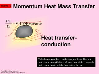
Residence Time Distribution MHMT8 Solution of Navier Stokes equation enables to calculate residence times of particles flowing through a continuous system. Residence time is in fact exposition time (exposition to temperature, radiation, catalyser,…) determining yield of chemical/biochemical reactions. First of all, experimentally determined residence time distribution is a diagnostics tool of continuous apparatuses.
Residence Time Distribution OUTLET INLET Fast particle (short residence time) MHMT8 Residence time = time spend by a particle inside a continuous system (time between entering and leaving the system). Let us assume that at a time interval (0,dt) we analyze all fluid particles passing through outlet and that we evaluate their residence times by backtracking streamlines using solution of Navier Stokes equations, or experimentally. Histogram of residence times of the collected particles is an important characteristic of continuous system, RTD-residence time distribution: RTD Residence time distribution E()= histogram of residence times of all particles passing through outlet. E()d is relative amount of particles having residence times within the interval (,+d).
RTD of circular pipe dr inlet outlet u(r) R r L Example: Laminar velocity profile for Newtonian liquid Mean residence time is the ratio of active internal volume and flowrate MHMT8 Let us consider as a system a straight pipe with fully developed velocity profile u(r). Streamlines are horizontal lines, and residence times =L/u(r) depend only upon the radial coordinate of fluid particles. Distribution of residence times is determined by the shape of velocity profile u(r): Radius r must be expressed as a function of , according to velocity profile Remark: Active volume cannot be evaluated just only from geometry of apparatus, because it is necessary to eliminate “dead” or stagnant regions, problems are with active volume of fixed porous beds etc. Measurement of mean residence time is usually the only way how to determine the active internal volume of continuous apparatuses.
RTD of circular pipe The result holds only for the residence time >min where min is the shortest residence time of the fastest particle moving at axis (min is sometimes called the time of the first appearance). For the parabolic velocity profile when the maximum velocity is twice the mean velocity MHMT8 because E() is distribution mean residence time
RTD=E(t) Impulse response of a system MHMT8 Let us assume that during an infinitely short time interval (0,dt) are all particles passing through inlet labeled (for example exposed to a short flash of light). Detector located at outlet counts at a time t the labeled particles (these particles have residence time within the interval (t,t+dt)) and their concentration is proportional to E(t). Normalised time response recorded by the detector is therefore identical with the residence time distribution E(t) (which is frequently called impulse response). L Experiments: Instantaneous labeling of fluid particle is usually realised by a very short injection of tracer (radionuclide, solution of salt,…) into the inlet stream, and concentration of tracer at outlet(impulse response) is recorded by a suitable transducer (Geiger Muller counter, conductivity probe,…). Remark: Later on we shall analyze the diffusion of tracer in more details (Axial Dispersion Model in the last lecture on mass transport)
RTD=E(t) Impulse response of a system MHMT8 Mathematically: The impulse response E(t) is the response of a general system to infinitely short pulse (→0) having unit area (Dirac delta function). Delta function (t) is zero for t≠0 and In this way the residence time distribution E(t) can be evaluated theoretically by solving transient transport equations for a “tracer” concentration with boundary condition at inlet prescribed in form of a short pulse of concentration. 1/ E(t) t [s]
Example response of system to a pulse (1/3) Derive response cout(t) of a perfectly mixed tank of inner volume V to a short pulse of tracer concentration cin(t) Initial condition: zero concentration c in the tank at time t=0. ? 0 t[s] Constant flowrate at inlet 0 t[s] Concentration in tank is the same as at outlet (perfect mixing, concentration is uniform inside) Constant flowrate at outlet MHMT8
Example response of system to a pulse (2/3) 0 t[s] Mean residence time MHMT8 First step – describe the system by differential equation for concentration c(t) in the mixed tank Mass balance of tracer (concentration c in the perfectly mixed tank)
Example response of system to a pulse (3/3) MHMT8 Response to a unit step stimulus function cin(t)=1 (up to the time ) Response to zero concentration at inlet for t> (initial concentration )
RESPONSE of a system to arbitrary stimulus cin() E(t-) E(t-)cin()d d t [s] MHMT8 An arbitrary function cin() can be substituted by a series of infinitely short rectangular pulses. Response to a pulse acting at time is the shifted impulse response E(t-) multiplied by the area of pulse. Response of system to all pulses is the integral: To understand the second integral use substitution t-=*
F(t)-integral distribution Inlet is switched to „red“ tracer since the time 0. L MHMT8 Inlet concentration in form of unit step (Heaviside function-integral of Dirac delta function) results to the concentration response expressed as the convolution integral Relationship between the impulse response and F-distribution Experiments: Inlet stream is switched to the tracer stream since the time 0. Concentration of tracer at outlet is proportional to the integral distribution F(t). The value F(t) is the ratio of flowrate of the particles having residence time less then t to the overall flowrate.
F(t) of circular pipe MHMT8 Example: Stabilised laminar parabolic profile in a circular tube results to the integral distribution of residence times (derived from the known impulse response E(t)) Application: Let us consider an extruder producing coloured fibers (spinning). For how long the quality of product will be decreased by ingredients of old colour after switching to a new colour? The F(t) graph indicates that as soon as 25% of “old” colour is tolerated (F=0.75) this time is 1 s (or more precisely ).
F(t) of circular pipe MHMT8 Example: Integral residence time distribution F(t) for stabilised laminar power-law velocity profile (n-flow behaviour index) in a circular tube inlet outlet R r n=1 L n=0.5 Relationship between radius and residence time t=L/u(r)
EXAM MHMT8 Residence time distribution
What is important (at least for exam) MHMT8 Definition of RTD and impulse response Distribution, mean residence time Integral distribution
What is important (at least for exam) MHMT8 Stimulus response relationship. Convolution