Acoustic modeling
Acoustic modeling (AM) is a crucial component in speech recognition systems, leveraging stochastic models to determine the probability of linguistic events based on sequences of feature vectors extracted from speech signals. Hidden Markov Models (HMMs) are utilized for their flexibility, accuracy, and efficiency. Originally proposed by Markov in 1913, HMMs enable effective training and have applications beyond speech, including pattern recognition and linguistic analysis. This overview explains the foundational concepts of HMMs, their properties, and their application in ASR, offering insights into the underlying mechanics of these models.

Acoustic modeling
E N D
Presentation Transcript
Hidden Markov Models • Acoustic models are stochastic models used with language models and other models to make decisions based on incomplete or uncertain knowledge. Given a sequence of feature vectors X extracted from speech signal by a front end, the purpose of the AM is to compute the probability that a particular linguistic event (word, sentence, etc.) has generated the sequence • AM have to be flexible, accurate and efficient -> HMMs are! • easy training • First used by Markov(1913) to analyse the letter sequence in a text • efficient method of training proposed by Baum et al. (1960) • application to ASR - Jellinek (1975) • application also in other areas: pattern recognition, linguistic analysis (stochastic parsing)
HMM Theory First order Markov hypothesis • HMM can be defined as a pair of discrete time stochastic processes (I,X). The process I takes values from a finite set I, whose elements are called states of the model, while X takes values in a space X that can be either discrete or continuous, depending on nature of data sequences to be modeled and is called observation space • The processes satisfy following relations, where right-hand probabilities are time t independent • history before time t has no influence on the future evolution of the process if the present state is specified • neither evolution of I nor past observations influence the present observation if the last two states are specified; output probabilities at time t are conditioned by states of I at time t-1 and t, i.e. by the transition at time t • random variables of process X represent the variability of the realization of the acoustic events, while process I models various possibilities in the temporal concatenation of these events Output independence hypothesis
HMM theory 2 • Properties of HMMs: • 0<=s <= t <= T, h>0 • The probability of every finite sequence X1T of observable random variablescan be decomposed as: • From these follows that HMM can be defined by specifying parameter set V=(P,A,B), where • P =Pr(I0=I) is the initial state density • aij=Pr(It=j|It-1=I) is the transition probability matrix A • bij=Pr(Xt=x|It-1=I, It=j) is the output densities matrix B • the parameters satisfy the following relation: • thus model parameters are sufficient for computing the probability of a sequence of observations, (but usually faster formula used)
HMMs as a probabilistic automata HMM • Nodes of graph correspond to states of Markov chain, while directed arcs correspond to allowed transtions aij • A sequence of observation is regarded as an emission of the system which at each time instant makes a transition form one to another node randomly chosen according to a node-specific probability density and generates a random vector according to arc-specific probability density. A number of states and set of arcs is usually called model topology. • In ASR it is common to have left-to-right topologies, in which aij=0 for j<I • also usually first and last states are not-emitting, i.e. source and final states are for setting initial and final probabilities, empty transitions needs slight modification of the algorithm Typical phone model topology
HMM is described by: • Observation sequence O=O1...OT • States sequence Q=q1...qT • HMM states S={S1...SN} • Symbols (emissions) V={v1...vm} • Transition probabilities A • Emission probabilities B • Initial state density P • Parameter set l=(A,B,P)
Example: wether • States: S1 – rain, s2- clouds, s3- sunny • observed only by the temperature T (density function different for diferrent states) • What is the probabilty of observed temperature sequence (20,22,18,15)? • Which sequence of states (rain, clouds, sunny) is the most probable? O={O1=20o, O2=22o, O3=18o, O4=15o} and start is sunny Following state seqeunces are possible: Q1={q1=S3, q2=S3,q3=S3,q4=S1}, Q2={q1=S3, q2=S3,q3=S3,q4=S3}, Q3={q1=S3, q2=S3,q3=S1,q4=S1}, etc. s1 s1 s2 s3 a31 Emission probabilities B Transition probabilities A
Weather II • For each state sequence the conditional probability can be found which depends on observation sequence: assuming O={O1=20o, O2=22o, O3=18o, O4=15o} and start is sunny Q1={q1=S3, q2=S3,q3=S3,q4=S1}, Q2={q1=S3, q2=S3,q3=S3,q4=S3}, Q3={q1=S3, q2=S3,q3=S1,q4=S1}, etc. Generally, the observed temperature sequence O can be generated by many state sequences which are not observable. The probability of temperature sequence given a model is
Trellis for weather P1b1(O1) P2b2(O1) P3b3(O1) a22 a12 a32 + *b2(O2) O = O1 O2 O3 O4 O5 a31 s1 s1 s2 s3 • Init: • Iterations: • Final step:
Left-right models: SR • Init: • Iterations: • Final: • For speech recognition: • left to right models • Find best path in trellis • Instead of summation take max –the path will give the best sequence of states – the most probable state sequence • An additional pointers array is needed to store best pathes • Backpointers show the optimal path
Training- estimation of model parameters • Count the frequency of occurences to estimate bj(k) • Transition probabilities: • Assumption: we can observe states of the HMM, what not always is possible: solution: forward-backward training
Forward/Backward training • We cannot observe state sequences, but we can compute expected values depending on model parameters, iterative estimation (new params with – above)
Forward-Backward 2 a31 s1 s1 s2 s3 • Forward probability: • Backward probability i.e. prob of Ot+1..OT ending in state Si • Iterative computation of backward probability: P1b1(O1) P2b2(O1) P3b3(O1) a21 a12 a31 + *b2(O2) O O Si O O = O1 Ot-1 Ot Ot+1 Ot+1 O at+1(j) aijbj(Ot+1) O Sj O bt+1(j)
FB 3 • Now compute the probability that the model in tact t is in the state si • The formula gives the probability of being in the state i in the tact t, but we need additionally the expected value of tacts spend in the state i and expected number of transitions • For ergodic processes (doesn’t depend on time), assuming sequence X=x1,x2,..xi,..,xT with only discrete values (e.g. {a,b,c})
FB 5 • The estimation procedure is done iteratively, so that P(O,lnew) >= P(O,l) • The previous equations assume single observations, what for multiple? • Let O={O(1),O(2), .. O(M)} be the training examples • {O(m)} are statistically independent, thus: • This could be solved this way, that we introduce a fictive observation in which all observations are concatenated together • Than we have
HMM: forward and backward coefficients • Additional probabilities have been defined to save computational load • two effectiveness goals: modelparameter estimation and decoding (search, recognition) • Forward probability is the Pr that X emits the partial sequence x1t and process I in state i at time t: • can be iteratively computed by: • backward probability is the Pr that X emits the partial sequence xt+1T and process I in state i at time t: • best-path probability is the maximum joint probability between partial sequence x1t and state sequence ending at state I at time t
Total probability: Trellis • Total probability of an observation sequence can be computedas: • or using v which measures the probability along the path which gives the highest contribution to the summation: • these algorithms have a time complexity o(MT), where M is the number of transition with non-zero probability (depends on the number of states in system N) and T is the length o input sequence • the computation of these probabilities is performed in a data structure called trellis, which corresponds to unfolding of time axis of the graph structure Trellis Dashed arrows - paths which score is added to obtain a probability, dotted for b, v corresponds to the highest scoring path among dashed ones
Trellis 2 • Nodes in the trellis are pairs (t,i) t-time index, i - model state, arcs represent model transitions composing possible path in the model; for given observation x1T each arc (t-1,I) -> (t,j) carries a “weight” given by aijbij(xt) • then for each path a score corresponding to the products of the weights of the arcs traversed by the path can be assigned. This score is the probability of emission of the observed sequence along the path, given v, current set of model parameters • formulas left • the recurrent computation of a,b, vcorresponds to appropriate combination at each trellis node, the scores of paths ending or starting at that node • the computation proceeds in a column-wise manner, synchronously with the apperance of observations. At every frame the scores of the nodes in a column are updated using recursion formula which unvolve the values of an adjacent column, transition probabilities of the models and the values of output denities for the current observation • for a and v computation starts from left column whose values are initialized by p and ends at outermost right column where the final value is computed. For b computations go in opposite direction
Output probabilities • If the observation sequences are composed of symbols drawn from a finite alphabet of O symbols, then a density is a real valued vector [b(x)]x=1O having a probability entry for possible symbol with the constraints: • observation may be also composed of couple of symbols, usually considered to be mutually statistically independent. Then the output density can be represented by the product of Q independent densities . Such a models are called discrete HMMs • discrete HMMs are simpler - only array access to find b(x), but imprecise, thus in current implementations rather continuous densities are used • to reduce memory requirements parametric representations are used • most popular choice: multivariate Gaussian density: where D is the dimension of vector space (length of a feaure vector). Parameters of Gaussian density are: mean vector m (location parameter) and symmetric covariance matrix S (spread of values around m) • widespread in statistics, parameters easy to estimate
Forward algorithm • To calculate the probability (likelihood) P(X|l) of the observation sequence X=(X1,X2,...XT) given the HMM l the most intuitive way is to sum up the probabilities of all state sequences: • In other words, first we enumerate all possible state sequences S of length T, that generate observation X and sum all the probabilities. The probabiloity of each path S is the product of the state sequence probability and joijnt output probability along the path. Using output-independence assumption • So finally we got: • First we enumerate all possible state sequences with length T+1. For any given state sequence we go through all transitions and states in a sequence until we reach the last transition – this require O(NT) state sequences generation – exponential computational complexity
Forward algorithm II - Trellis • Based on the HMM assumption that P(st|st-1,l) P(Xt|st,l) involves only st-1, st P(X|l) can be computed recursively using so called forward probabilityat(i)=P(X1t,st=i | l) denoting partial probability that HMM is in state i having generated partial observation X1t (i.e. X1..Xt) • This can be illustrated by trellis: arrow is the transition from state to state, number within circle denotes a. We start a cells from t=0 with initial probabilities, other cells are computed time-synchroneous from left to right where each cell is completely computed before proceeding to time t+1, When the states in the last column have been computed, the sum of all probabilities in the final column is the probability of generating the observation sequence
Gaussians • Disadvantage: Gaussian densities are unimodal: to overcome this Gaussianmixtures are used (weighted sums of Gaussians) • mixtures are capable to approximate other densities using appropriate number of components • D-dimensional Gaussian mixture with K components can be described using K[1+D+(D(D+1)/2)] real numbers (D=39, K=20 then 16400 real numbers) • further reduction: diagonal covariance matrix (components mutually independent). The joint density is then the product of one-dimensional Gaussian densities corresponding to the individual vector elements - 2D parameters • diagonal-covariance Gaussians are widely use in ASR • to reduce number of Gaussians: distribution tying or sharing is often used: imposing that different transitions of different models share the same outout density. The tying scheme exploits a priori knowledge, e.g. sharing densities among allophones or sound classes (will be in details described further) • attempts to use other densities known from literature: Laplacians, lambda densities (for duration), but Gaussians dominate
HMM composition • Probabilistic decoding: ASR with stochastic models choosing in the set of the possible linguistic events the one that corresponds to the observed data with the highest probability • in ASR an observation often does not correspond to the utterance of a single words, but of a sequence of words. If the language has a limited set of sentences, then it is possible to have models for each utterance, but what to do if the number is unlimited? To much models are also not easy to handle, how to train them, impossible to recognize items not observed in training material • solution: concatenation of units from a list of manageable size, describe training Model linking
DTW • Warp two speech templates x1..xN and y1..yM with minimal distortion: to find the optimal path between starting point (1,1) and end point (N,M) we need to compute the optimal accumulated distance D(N,M) based on distances d(i,,j). Since the same optimal path must be based on the previous step, the minimum distance must satisfy following equation:
Dynamic programming algorithm • We need only consider and keep only the best move for each pair although tehre are M possible moves, DTW can be computed recursively • We can identify the optimal match yj with respect to xi and save the index in a back pointer table B(i,,j)
Viterbi algorithm • We are looking for the state sequence S=(s1,s2..sT) that maximizes P(S,X|l) – very similiar to dynamic programming (for forward probabilities). Instead of summing up probabilities from different paths coming to the same destination state, the Viterbi algorithm picks and remember the best path. Best path probability is defined as: • Vt(i) is the probability of the most likely state sequence at time t which has generated the observation X until time t and end in state i.
Viterbi algorithm • Algorithm for computing v probabilities- application of dynamic programming for finding a best scoring path in a directed graph with weighted arcs, I.e. in trellis • one of the most important algorithms in current computer science • uses recursive formula • when the whole observation sequence x1T has been processed, the score of the best path can be found computing: • identity of states can be attained using backpointers f(x,I) - this allows to find optimal state sequence: this constitutes a time alignment of input speech frames, allowing to locate occurrences of SR units (phonemes) • construction of recognition model: • first the recognition language is represented as a network of words (‘finite-state automata’). The connection between words are empty transitions, but could have assigned probability (LM, n-gram) • each word is replaced by a sequence (or network) of phonemes according to lexical rules. • Phonemes are replaced by instances of appropriate HMMs. Special labels are assigned to word-ending states (simplifies retrieving word sequence)
Vitterbi movie • The Viterbi algorithm is an efficient way to find the shortest route through a type of graph called a trellis. The algorithm uses a technique called 'forward dynamic programming' which relies on the property that the cost of a path can be expressed as a sum of incremental or transition costs between nodes adjacent in time in the trellis. The demo shows the evolution of the Viterbi algorithm over 6 time instants. At each time the shortest path to each node at the next time instant is determined. Paths that do not survive to the next time instant are deleted/ By time k+2, the shortest path (track) to time k has been determined unambiguously. This is called 'merging of paths'. states
Viterbi pseudocode • note use of stack
Model choice in ASR • Identification of basic units is complicated due to various NL effects: reduction, other pronunciation depending on context, etc. Thus, sometime phoneme are not appropriate representation • better: use context-dependend units: allophones • triphones: context made by previous and following phonemes (monophones) • phoneme models can have left-to-right topology with 3 groups of states: onset, body and coda • note the huge number of possible triphones: 403=64000 models! Of course not all occurs due to phononatctic rules, but: How to train? How to manage? • Other attempts: half-syllables, diphones, microsegments, etc.but all methods of unit selection base on a priori phonetic knowledge • totally different approach: automatic unsupervised clustering of frames. Corresponding centroids are taken as starting distributions for a set of basic simple units called fenones. Maximum likelihood decoding of utterances in terms of fenones is generated (dictionary) and fenones are then combined to built word models and the models are then trained The shared parameter (i.e., the output distribution) associated with a cluster of similar states is called a senone because of its state dependency. The phonetic models that share senones are shared-distribution models or SDM's Fenone
Parameter tying yes no • good trade-off between resolution and precision of models, imposing an equivalence relation between different components of the parameter set of the models or components of different models • definition of tying relation: • involves decision about every parameter of the model set • a priori knowledge-based equivalence relations : • semi-continuous HMMs: set of output density mixtures which shares the same set of basic Gaussian components (SCHMMs) - they differ only by weights • phonetically tied-mixtures: set of context-dependent HMMs in which the mixtures of all allophones of a phonem share a phoneme-dependent codebook • state-tying: clustering of states based on similarity of Gaussians (Young & Woodland, 94) and retraining • phonetic decision trees (Bahr et al, 91): binary decision tree which has a question and a set of HMM densities attached to each node; questions generally reflect phonetic context, e.g. “is the left context a plosive?” • genones: automatically determined SCHMMs : 1. Mixtures of allophones are clustered - mixtures with common components identified 2. Selecting of most likely elements of clusters: genones 3. Retraining of the system Mostly used
Implementation issues • Overflow and underflow during computations may occur - the probabilities are very small, especially for long sentences - to overcome this log are used