Download
1 / 27
300 likes | 750 Vues
Gaussian Mixture Models and Acoustic Modeling. Lecture 9 Spoken Language Processing Prof. Andrew Rosenberg. Acoustic Modeling. The goal of the Acoustic Model is to hypothesize a phone label based on acoustic observations .

E N D
Gaussian Mixture Models and Acoustic Modeling Lecture 9 Spoken Language Processing Prof. Andrew Rosenberg
Acoustic Modeling • The goal of the Acoustic Model is to hypothesize a phone label based on acoustic observations. • The phone label will be defined by the phone inventory (e.g., IPA, ARPAbet, etc.) • Acoustic Observations will be MFCCs • There are other options.
Mixture Models • A Mixture Model is the weighted sum of a number of pdfs where the weights are determined by a multinomial distribution, π
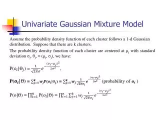
Gaussian Mixture Model • GMM: weighted sum of a number of Gaussians where the weights are determined by a multinomial, π
Latent Variable representation • The mixture coefficients can be viewed as a latentor unobservedvariable. • Training a GMM involves learning both the parameters for the individual Gaussian Models and the Mixture coefficients. • For a fixed set of data points x, the optimal setting of the GMM parameters may not have a single optimum.
Maximum Likelihood Optimization • Likelihood Function • Log likelihood • A log transform makes the optimization much simpler.
Optimizing GMM parameters • Identifying the optimal parameters involves setting partial derivatives of the likelihood function to zero.
Optimizing GMM parameters • Covariance Optimization
Optimizing GMM parameters • Mixture Term
What’s the problem? • Circularity: The responsibilities are assigned by the GMM parameters, and are used in identifying their optimal settings • The Maximum Likelihood Function of the GMM does not have a closed for optimization for all three variables. • Expectation Maximization: • Keep one variable fixed, optimize the other. • Here, • fix the responsibility terms, optimize the GMM parameters • then fix the GMM parameters, and optimize the responsibilities
Expectation Maximization for GMMs • Initialize the parameters • Evaluate the log likelihood • Expectation-step: Evaluate the responsibilities • Maximization-step: Re-estimate Parameters • Evaluate the log likelihood • Check for convergence
E-M for Gaussian Mixture Models • Initialize the parameters • Evaluate the log likelihood • Expectation-step: Evaluate the responsibilities • Maximization-step: Re-estimate Parameters • Evaluate the log likelihood • Check for convergence
EM for GMMs • E-step: Evaluate the Responsibilities
EM for GMMs • M-Step: Re-estimate Parameters
Potential Problems • Incorrect number of Mixture Components • Singularities
Singularities • A minority of the data can have a disproportionate effect on the model likelihood. • For example…
Singularities • When a mixture component collapses on a given point, the mean becomes the point, and the variance goes to zero. • Consider the likelihood function as the covariance goes to zero. • The likelihood approaches infinity.
Training acoustic models • TIMIT • close, manual phonetic transcription • 2342 sentences • Extract MFCC vectors from each frame within each phone • For each phone, train a GMM using Expectation Maximization. • These GMM is the Acoustic Model. • Common to use 8, or 16 Gaussian Mixture Components.
Sequential Models • Make a prediction every frame. • How often can phones change? • Encourage continuity in predictions. • Model phone transitions.
Next Class • Hidden Markov Models • Reading: J&M 5.5, 9.2