Download
1 / 11
120 likes | 806 Vues
Univariate Gaussian Mixture Model. Assume the probability density function of each cluster follows a 1-d Gaussian distribution. Suppose that there are k clusters.

E N D
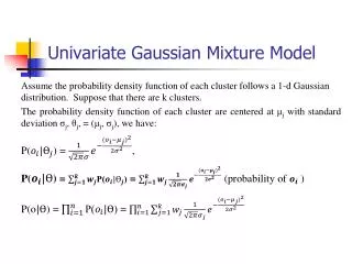
Univariate Gaussian Mixture Model Assume the probability density function of each cluster follows a 1-d Gaussian distribution. Suppose that there are k clusters. The probability density function of each cluster are centered at μj with standard deviation σj, θj, = (μj, σj), we have: P() = , P() == (probability of ) P(o) ==
Simple Mixture Model Assume there are two Gaussian distributions, with a common standard deviation(σ) of 2 and means(μ) of -4 and 4, respectively. Also assume that each of the two distributions is selected with equal probability, i.e.,= =0.5. So the probability of an object o is given: P(o) =
Distribution 1 Distribution 2 (a) Probability density function for the mixture model (b) 20,000 points generated from the mixture model • Mixture model consisting of two normal distributions with means of -4 and 4, respectively. Both distributions have a standard deviation of 2. • P() =
Univariate Gaussian Mixture Model • Given n objects O = {o1, …, on}, we want to mine a set of parameters = {θ1, …, θk} s.t.,P(o|) is maximized, where θj = (μj, σj) are the mean and standard deviation of the j-thunivariate Gaussian distribution • We initially assign random values to parameters θj, then iteratively conduct the E- and M- steps until converge or sufficiently small change • At the E-step, for each object oi, calculate the probability that oi belongs to each distribution, P(, ) = • At the M-step, adjust the parameters θj = (μj, σj) so that the expected likelihood P(o|) is maximized • ==,
EM algorithm • Select an initial set of model parameters. • Repeat • E-Step: for each object, calculate the probability that each object belongs to each distribution, i.e., calculate P(, ) • M-Step: given the probabilities from E-Step, find the new estimates of the parameters that maximize the expected likelihood. • Until The parameters do not change. • (Alternatively, stop if the change in the parameters is below a specified threshold)
A Simple Example of EM Algorithm Consider the previous distributions, we assume that we know the standard deviation(σ) of both distributions is 2.0 and that points were generated with equal probability from both distributions. We will refer to the left and right distributions as distributions 1 and 2, respectively. Distribution 1 Distribution 2
Initialize Parameters and E-Step We can begin with μ1= -2 andμ2= 3. Thus, the initial parameters, = (μ,σ), for the two distributions are, respectively and .The set of parameters for the entire mixture model is = {} For the Expectation Step of EM, we want to compute the probability that a point came from a particular distribution; i.e., we want to compute P(, ) andP(, ) . These values can be expressed by the following equation, which is a straightforward application of Bayes rule: P(, ) =, here we have only 2 distributions and each weight w is 0.5, so: P(, ) =
Expectation Step of EM For instance, assume one the points is 0. We can calculate the p(0|) according to Gaussian density function: P() = , and we also know that and , P(0) == = 0.12 P(0)== 0.06 Then use P(, ) = to calculate P(|0, ) and P(|0, ) : P(|0, ) = 0.12/(0.12+0.06) = 0.66 P(|0, ) = 0.06/(0.12+0.06) = 0.33
Expectation Step of EM We can see that for point 0, P(|0, ) = 0.66 and P(|0, ) = 0.33, which means that the point 0 is twice likely to belong to distribution 1 as distribution 2 based on the current assumptions for the parameter values. And in Expectation Step of EM, we need to calculate P(, )for each object. (P(, )means the probability that each object belongs to each distribution) So for this case, we need to compute the cluster membership probabilities for all 20,000 points. After the calculation, the E-Step of the first iteration is over.
Maximization Step of EM After computing the probabilities for all 20,000 points, we need to find the new estimators for and in the M-Step of EM. We use these equations: ==, For instance, compute the new and : == = -3.74 == = 4.10
First few iterations of EM We repeat these E-Step and M-Step until the estimates of and either don’t change or change very little. The table above gives the first few iterations of EM algorithm when it is applied to the set of 20,000 points.