Approximating The Kullback-Leibler Divergence Between Gaussian Mixture Models

1. Approximating The Kullback-Leibler Divergence Between Gaussian Mixture Models ICASSP 2007 John R. Hershey and Peder A. Olsen IBM T. J. Watson Research Center Speaker: 孝宗

2. Outline • Introduction • Kullback-Leibler Divergence • Methods • Monte Carlo Sampling • The Unscented Transformation • Gaussian Approximations • The Product of Gaussian Approximation • The Matched Bound Approximation • The Variational Approximation • The Variational Upper Bound

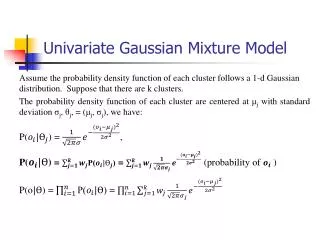
3. Introduction • Kullback-Leibler Divergence: relative entropy • KLD between two PDF and • Three properties: • Self similarity: • Self identification: • Positivity:

4. Introduction • The KL divergence is used in many aspects of speech and image recognition, such as determining if two acoustic models are similar,[2], measuring how confusable two words or HMMs are, [3, 4, 5] • For two Gaussians and the KLD has closed formed expression, • Whereas for two GMMs no such closed form expression exists.

5. Monte Carlo Sampling • The idea is to draw a sample from the pdf such that • Using n i.i.d. samples we have ( if f(x) is PDF) • To draw a sample from a GMM we first draw a discrete sample according to the probabilities . Then we draw a continuous sample from the resulting gaussian component

6. The Unscented Transformation 1.Choise sigma point 2.Each sigma points has a weight 4. Compute a Gaussian from weighted points 3. Non-linear transform http://ais.informatik.uni-freiburg.de/teaching/ws12/mapping/pdf/slam05-ukf.pdf

7. The Unscented Transformation • An approach to estimate in such a way that approximation is exact for all quadratic function • It is possible to pick up 2d sigma points such that • One possible choice of the sigma points is

8. The Unscented Transformation

9. Gaussian Approximations • Replace and with Gaussians • Another method :

10. The Product of Gaussian Approximation • The likelihood defined by So…

11. The Product of Gaussian Approximation *Jensen’s Inequality 因為log是concave function

12. The Product of Gaussian Approximation • Closed-form solution • Self similarity • Self identification  • Positivity • tends to greatly underestimate (Jensen’s Inequality)

13. The Matched Bound Approximation • If and have the same number of components Log-sum inequality 為1

14. The Matched Bound Approximation • Goldberger’s approximate formula • Define a match function, • Self similarity • Self identification  • Positivity 

15. The Variational Approximation • Define variational parameters such that • We get the best bound by maximizing with respect to . Lower bound

16. The Variational Approximation Define: For equal numbers of components, if we restrict and to have only one non-zero element for a given a, the formula reduces exactly to the chain rule upper bound given in equation (13).

17. The Variational Upper Bound • Define satisfying the constraints , • With this notation we use Jensen’s inequality to obtain an upper bound of the KL divergence as follows

18. The Variational Upper Bound • finding the variational parameters that minimize • The problem is convex in as well as inso we can fix one and optimize for the other • Since any zero in and are fixed under the iteration we recommend starting with

19. Experiments • the acoustic model consists of a total of 9,998 gaussiansbelonging to 826 separate GMMs. The number of gaussians per GMM varies from 1 to 76, of which 5 mixtures attained the lower bound of 1. • The median number of gaussians per GMM was 9. We used all combinations of these 826 GMMs to test the various approximations to the KL divergence.

20. Experiments • Each of the methods was compared to the reference approximation, which is the Monte Carlo method with one million samples, denoted DMC(1M). • The vertical axis represents the probability derived from a histogram of the deviations taken across all pairs of GMMs.

21. Experiments

22. Experiments

23. Conclusion • If accuracy is the primary concern, then MC is clearly best. • when computation time is an issue, or when gradients need to be evaluated, the proposed methods may be useful. • Finally, some of the more popular methods, , , and , should be avoided, since better alternatives exist.