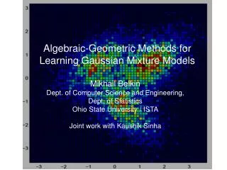
Algebraic-Geometric Methods for Learning Gaussian Mixture Models
Algebraic-Geometric Methods for Learning Gaussian Mixture Models. Mikhail Belkin Dept. of Computer Science and Engineering, Dept. of Statistics Ohio State University / ISTA Joint work with Kaushik Sinha. TexPoint fonts used in EMF.

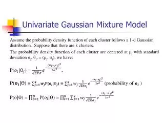
Algebraic-Geometric Methods for Learning Gaussian Mixture Models
E N D
Presentation Transcript
Algebraic-Geometric Methods for Learning Gaussian Mixture Models Mikhail Belkin Dept. of Computer Science and Engineering, Dept. of Statistics Ohio State University / ISTA Joint work with KaushikSinha TexPoint fonts used in EMF. Read the TexPoint manual before you delete this box.: AAAAAAAAAAAAAAAAAAA
From crabs to Gaussians First considered by Pearson, 1894. Analyzed 1000 crabs from Naples. Concluded (erroneously?) that there were two distinct populations.
The Problem Learning Gaussian Mixture Model • Classical problem in statistics • goes back to the classical work of Pearson(1894) . • Widely used model for scientific/engineering tasks • Application areas include • Speech Recognition • Computer Vision • Bioinformatics • Astronomy • Medicine • …..
Gaussian Mixtures Problem: identifying parameters of a Gaussian mixture distribution from a finite sample. The Problem
The Problem The Problem • Mixture of Gaussians in • What does learning such a mixture mean? • estimating the parameters of a mixture within pre-specified accuracy from a sample. • parameters are the means, covariance matrices and mixing weights of component Gaussian distributions. • number of parameters:
Most popular method: Expectation Maximization EM is by far the most popular method for mixture fitting. Iterative procedure to find parameters (similar to k-means clustering). Simple to implement. Guaranteed to converge. Converges to true values, if initialized close to true values. However: Sensitive to initialization. Numerous local maxima. Does not detect the number of components. Expectation Maximization
How EM fails: a simple example From Tao, Belkin, Yu, Annals of Statistics, 2010
The Problem Some Recent Progress • Understanding computational aspects of Gaussian Mixture Learning • is it possible to learn Gaussian mixture in time and using a sample of size polynomial in dimension? • Dasgupta (1999) showed that learning a mixture of Gaussians in using a sample size polynomial in n is possible. • result was surprising because complexity of many problems scales exponentially with dimension (curse of dimensionality). Something as simple as the volume of a convex body cannot be estimated using number of samples polynomial in dimension (Barany, Furedi, 88).
Learning in high dimension Dasgupta’s Result, 1999 • It is possible to learn mixture of Gaussians in using a sample size polynomial in , if the component separation is rof the order • component separation is the minimum distance between the component means.
Summary of Existing Results Partial Summary of Results on Gaussian Mixture Learning • Min. separation is independent of and • Our Result (solves the general problem)
Summary of Existing Results Partial Summary of Results on Gaussian Mixture Learning • Min. separation is independent of and • Our Result (solves the general problem) Min. separation is an increasing function of and/orr
Summary of Existing Results Partial Summary of Results on Gaussian Mixture Learning • Min. separation is independent of and • Our Result (solves the general problem) Min. separation is an increasing function of and/orr
Summary of Existing Results Partial Summary of Results on Gaussian Mixture Learning • Min. separation is independent of and • Our Result (solves the general problem) Min. separation is an increasing function of and/orr
Obstacle in Learning Identifiabilty • Different values of parameters could give rise to same distribution • Need for a quantification of how hard it is to learn the parameters from data Example: parameters of the following distribution family cannot be learned from sampled data
Obstacle in Learning Identifiabilty • Different values of parameters could give rise to same distribution • Need for a quantification of how hard it is to statistically learn the parameters from data Example: parameters of the following distribution family cannot be learned from sampled data
Obstacle in Learning Identifiabilty • Different values of parameters could give rise to same distribution • Need for a quantification of how hard it is to statistically learn the parameters from data Example: parameters of the following distribution family cannot be learned from sampled data If and are close to two values of parameters and with identical probability distributions , then it is hard to distinguish them from sampled data, even when is large. Example:
Radius of Identifiability Radius of Identifiability • Introduce Radius of Identifiability • it is the radius of largest open ball around such that any two different parameters from this ball give rise to different probability density functions. • if no such ball exists, i.e., , then parameters cannot be identified uniquely, given any amount of data. • complexity scales with
Radius of Identifiability Radius of Identifiability • Introduce Radius of Identifiability • it is the radius of largest open ball around such that any two different parameters from this ball give rise to different probability density functions. • if no such ball exists, i.e., , then parameters can not be identified uniquely, given any amount of data. • complexity scales with We show that explicit formula of for Gaussian mixture is
Our Result Main Result • We show that the parameters of a Gaussian mixture with radius of identifiability in can be learned (up to permutation) within pre-specified precision with confidence using a sample size , where is radius of the bounding ball. • minimum separation can even be zero, i.e., two Gaussian components can have same means but different covariance matrices. • polynomial dependence on is necessary.
Overview of Our Proof Overview of Our Proof • Reduction to fixed dimension • we show that learning Gaussian mixture in dimensions can be reduced to , parameter estimation problems in dimensions. (more on this later) • Learning in fixed dimension • we introduce the general notion of “polynomial family” (more on this soon). • we show that the parameters of polynomial families can be learned within accuracy with confidence at least , using a sample of size polynomial in dd and . • in addition to Gaussian distribution, almost all standard parametric probability distributions as well as their mixtures and products form polynomial families (more on this soon).
Overview of Our Proof Overview of Our Proof • Reduction to fixed dimension • we show that learning Gaussian mixture in dimensions can be reduced to , parameter estimation problems in dimensions (more on this later). • Learning in fixed dimension • we introduce the general notion of “polynomial family” (more on this soon). • we show that the parameters of polynomial families can be learned within accuracy with confidence at least , using a sample of size polynomial in dd and . • in addition to Gaussian distribution, almost all standard parametric probability distributions as well as their mixtures and products form polynomial families (more on this soon).
Overview of Our Proof Overview of Our Proof • Reduction to fixed dimension • we show that learning Gaussian mixture in dimensions can be reduced to , parameter estimation problems in dimensions (more on this later). • Learning in fixed dimension • we introduce the general notion of “polynomial family” (more on this soon). • we show that the parameters of polynomial families can be learned within accuracy with confidence at least , using a sample of size polynomial in dd and . • in addition to Gaussian distribution, almost all standard parametric probability distributions as well as their mixtures and products form polynomial families (more on this soon).
Polynomial Family Learning in Fixed Dimension: Polynomial Family • Definition • a family of probability distributions parameterized by , forms a polynomial family, if each (raw) moment of exists and can be represented as a polynomial of the parameters .
Polynomial Family Examples of Polynomial Families Gaussian Moments are given by Hermite Polynomials
Polynomial Family Examples of Polynomial Families Exponential Binomial Gaussian Gamma Moments are given by Hermite Polynomials Examples include almost all standard parametric families as well as their mixtures and products. Hence Gaussian mixtures are also a polynomial family.
Polynomial Family Proof Sketch For Learning in Fixed Dimension • Main result for polynomial families • there is an algorithm which given for an identifiable family , where is the set of parameters within a ball of radius , outputs within of with probability at least , using a number of sample points from polynomial in and . • Proof Sketch • given a polynomial family, find a finite set of moments that completely characterizes a distribution (identifiability). • reformulate the problem of learning the parameters in terms of this set of moments using algebraic inequalities. • reduce the problem of learning the parameters to 1 dimension, using techniques from algebraic geometry, specifically,Tarski-Seidenberg theorem (elimination of quantifiers).
Polynomial Family Identifiability and Finite Set of Moments • Identifiability • family is identifiable if for any . • We will prove that when is identifiable, finite number of moments are sufficient to uniquely identify the parameter (next slide) • Requires application of Hilbert Basis Theorem Hilbert Basis Theorem : Every ideal in a ring of polynomials is finitely generated.
Polynomial Family Finite Set of Moments Fully Characterizes Polynomial Family • For a polynomial family each moment is a polynomial of . • Let be a polynomial of variables. • Let be the ideal in the ring of polynomials of variables generated by polynomials . • Let , where is an increasing sequence. • Hilbert Basis theorem ensures that is finitely generated hence there exists some large enough such that for any • Identifiability implies first moments defines the distribution uniquely.
Polynomial Family Finite Set of Moments Fully Characterizes Polynomial Family • For a polynomial family each moment is a polynomial of . • Let be a polynomial of variables. • Let be the ideal in the ring of polynomials of variables generated by polynomials . • Let , where is an increasing sequence. • Hilbert Basis theorem ensures that is finitely generated hence there exists some large enough such that for any • Identifiability implies first moments defines the distribution uniquely.
Polynomial Family Finite Set of Moments Fully Characterizes Polynomial Family • For a polynomial family each moment is a polynomial of . • Let be a polynomial of variables. • Let be the ideal in the ring of polynomials of variables generated by polynomials . • Let , where is an increasing sequence. • Hilbert Basis theorem ensures that is finitely generated hence there exists some large enough such that for any • Identifiability implies first moments defines the distribution uniquely.
Polynomial Family Finite Set of Moments Fully Characterizes Polynomial Family • For a polynomial family each moment is a polynomial of . • Let be a polynomial of variables. • Let be the ideal in the ring of polynomials of variables generated by polynomials . • Let , where is an increasing sequence. • Hilbert Basis theorem ensures that is finitely generated hence there exists some large enough such that for any • Identifiability implies first moments defines the distribution uniquely.
Polynomial Family Finite Set of Moments Fully Characterizes Polynomial Family • For a polynomial family each moment is a polynomial of . • Let be a polynomial of variables. • Let be the ideal in the ring of polynomials of variables generated by polynomials . • Let , where is an increasing sequence. • Hilbert Basis theorem ensures that is finitely generated hence there exists some large enough such that for any • Identifiability implies first moments defines the distribution uniquely.
Polynomial Family Finite Set of Moments Fully Characterizes Polynomial Family • For a polynomial family each moment is a polynomial of . • Let be a polynomial of variables. • Let be the ideal in the ring of polynomials of variables generated by polynomials . • Let , where is an increasing sequence. • Hilbert Basis theorem ensures that is finitely generated hence there exists some large enough such that for any • Identifiability implies first moments defines the distribution uniquely.
Polynomial Family What Next? • If the first moments are known precisely then the problem of learning the parameters is almost solved • only remaining task is to solve a finite set of polynomial equations. • can be done algorithmically. • However, moments need to be estimated from sample data • uncertainty in moment estimation introduces uncertainty in parameter estimation. • how do we deal with it? • A powerful result from mathematics, called the Tarski-Seidenberg Theorem helps us to prove that • moment estimation error depends only polynomially on parameter estimation error.
Polynomial Family Tarski-Seidenberg Theorem • Semi-algebraic Set • a semi algebraic set in is a finite union of sets defined by a finite number of polynomial equations and inequalities. • Tarski-Seidenberg Theorem • Let be a projection map. If is a semi-algebraic set in for some ok , then is a semi-algebraic set in . • this is equivalent to elimination of quantifiers for semi-algebraic sets. Equivalent to elimination of existential quantifier
Polynomial Family Characterization of Uncertainty • Suppose first moments completely characterizes the distribution • for any two parameters , define . • , iff . • Fix and consider the set • since logical statements can be expressed as algebraic conditions by Tarski-Seidenberg Theorem is a semi-algebraic subset of . • eliminating the quantifiers reduces the problem to 1-dimension, where it can be shown that is polynomially dependent on supremum of .
Polynomial Family Characterization of Uncertainty • Suppose first moments completely characterizes the distribution • for any two parameters , define . • , iff . • Fix and consider the set • since logical statements can be expressed as algebraic conditions by Tarski-Seidenberg Theorem is a semi-algebraic subset of . • eliminating the quantifiers reduces the problem to 1-dimension, where it can be shown that is polynomially dependent on supremum of .
Polynomial Family Characterization of Uncertainty • Suppose first moments completely characterizes the distribution • for any two parameters , define . • , iff . • Fix and consider the set • here can be viewed as an around taking probability distribution into account. • since logical statements can be expressed as algebraic conditions by Tarski-Seidenberg Theorem is a semi-algebraic subset of . • eliminating the quantifiers reduces the problem to 1-dimension, where it can be shown that is polynomialy dependent on . • here can be viewed as an around taking probability distribution into account.
Polynomial Family A Simple Example • Consider a univariate Gaussian with zero mean • second moment uniquely defines this distribution. • For any two , assume and consider the following set • by Tarski-Seideberg Theorem is a semi algebraic subset of and in this case we can see what it is exactly (geometric interpretation on next slide). • For a fixed , supremum of represents allowable parameter estimation error for a fixed moment estimation error • elimination of and leads to a relation between and .
Reduction Reduction to Fixed Dimension • Results of learning polynomial families for a fixed dimension can not be applied directly to mixture of high-dimensional Gaussians • number of parameters to be estimated increases with dimension. • how do we deal with it? • We show that it is possible to estimate the parameters in high dimension by solving parameter estimation problems in appropriate low dimensions • why does it work?
Reduction Low-dimensional Projection of Gaussian Mixture • Some Good News • projecting a Gaussian mixture onto a lower dimensional coordinate plane yields a low-dimensional Gaussian mixture where, • mixing coefficients remain the same • new component means are the projections of the original component means, • new component covariance matrices are the restrictions of the original component covariance matrices. • results for polynomial families can be used to learn the parameters of this low-dimensional Gaussian mixture. • hopefully, parameters of high dimensional Gaussian mixture can be learned by learning the parameters of several low-dimensional Gaussian mixtures. • Some Difficulties • radius of identifiability of the projected gaussian mixture may become zero (not learnable!). • parameters of high dimensional Gaussian mixture may not be uniquely learned from the parameters of several low-dimensional Gaussain mixtures.
Reduction Low-dimensional Projection of Gaussian Mixture • Some Good News • projecting a Gaussian mixture onto a lower dimensional coordinate plane yields a low-dimensional Gaussian mixture where, • mixing coefficients remain the same. • new component means are the projections of the original component means. • new component covariance matrices are the restrictions of the original component covariance matrices. • results for polynomial families can be used to learn the parameters of this low-dimensional Gaussian mixture. • hopefully, parameters of high dimensional Gaussian mixture can be learned by learning the parameters of several low-dimensional Gaussian mixtures. • Some Difficulties • radius of identifiability of the projected Gaussian mixture may become zero (not learnable!). • parameters of high dimensional Gaussian mixture may not be uniquely learned from the parameters of several low-dimensional Gaussain mixtures.
Reduction Low-dimensional Projection of Gaussian Mixture • Good News • projecting a Gaussian mixture onto a lower dimensional coordinate plane yields a low-dimensional Gaussian mixture where, • mixing coefficients remain the same. • new component means are the projections of the original component means. • new component covariance matrices are the restrictions of the original component covariance matrices. • results for polynomial families can be used to learn the parameters of this low-dimensional Gaussian mixture. • hopefully, parameters of high dimensional Gaussian mixture can be learned by learning the parameters of several low-dimensional Gaussian mixtures.
Reduction Low-dimensional Projection of Gaussian Mixture • Some Difficulties • radius of identifiability of the projected Gaussian mixture may become zero (not learnable!). • parameters of high dimensional Gaussian mixture may not be uniquely learned from the parameters of several low-dimensional Gaussian mixtures.
Reduction Low-dimensional Projection of Gaussian Mixture • Some Difficulties • radius of identifiability of the projected Gaussian mixture may become zero (not learnable!). • parameters of high dimensional Gaussian mixture may not be uniquely learned from the parameters of several low-dimensional Gaussian mixtures.
Reduction Low-dimensional Projection of Gaussian Mixture • Some Difficulties • radius of identifiability of the projected Gaussian mixture may become zero (not learnable!). • parameters of high dimensional Gaussian mixture may not be uniquely learned from the parameters of several low-dimensional Gaussian mixtures.
Reduction Low-dimensional Projection of Gaussian Mixture • Some Difficulties • radius of identifiability of the projected Gaussian mixture may become zero (not learnable!). • parameters of high dimensional Gaussian mixture may not be uniquely learned from the parameters of several low-dimensional Gaussian mixtures.
Reduction Low-dimensional Projection of Gaussian Mixture • Some Difficulties • radius of identifiability of the projected Gaussian mixture may become zero (not learnable!). • parameters of high dimensional Gaussian mixture may not be uniquely learned from the parameters of several low-dimensional Gaussian mixtures. ?
Reduction Sketch of the algorithm • Step 1 • identify a low-dimensional (fixed) coordinate plane where radius of identifiability reduces only by a fixed amount. • this can be done deterministically by checking at most number of coordinate planes. • project high dimensional Gaussian mixture onto this coordinate plane and learn the parameters of this low-dimensional Gaussian mixture. • using results of learning polynomial families in a fixed dimension. • Step 2 • parameters along each remaining coordinate can be estimated separately by adding each coordinate at a time and aligning the estimates obtained from two parameter estimation problems in overlapping fixed dimensions. • total number of such low-dimensional parameter estimation problems is at most .
Reduction Sketch of the idea: two components in three dimensions.