Convolutional Networks: Operations and Motivations
Learn about convolution operation, sparse connectivity, parameter sharing, equivariant representations, pooling, and how convolutional networks leverage these concepts to improve machine learning systems. Discover the neuroscientific basis behind convolutional networks.

Convolutional Networks: Operations and Motivations
E N D
Presentation Transcript
Chapter 9Convolutional Networks Ruchengsen 2016.11.01
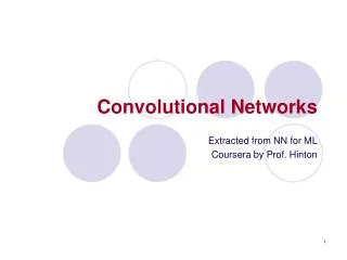
Convolutional networks are simply neural networks that use convolution in place of general matrix multiplication in at least one of their layers.
Outline • The Convolution Operation • Motivation • Pooling • Convolution and Pooling as an Infinitely Strong Prior • Variants of the Basic Convolution Function • Data Types • Random or Unsupervised Features • Structured Outputs • The Neuroscientific Basis for Convolutional Networks
The Convolution Operation The convolution operation is typically denoted with an asterisk: If we now assume that x and w are defined only on integer t, we can define the discrete convolution
The Convolution Operation In convolutional network terminology, the first argument (the function x) to the convolution is often referred to as the input and the second argument (the function w) as the kernel. The output is sometimes referred to as the feature map. If we use a two-dimensional image I as our input, we probably also want to use a two-dimensional kernel K: Convolution is commutative, meaning we can equivalently write:
Outline • The Convolution Operation • Motivation • Pooling • Convolution and Pooling as an Infinitely Strong Prior • Variants of the Basic Convolution Function • Data Types • Random or Unsupervised Features • Structured Outputs • The Neuroscientific Basis for Convolutional Networks
Motivation • Convolution leverages three important ideas that can help improve a machine learning system: • Sparse connectivity • Parameter sharing • Equivariant representations
Sparse connectivity • This is accomplished by making the kernel smaller than the input. • It stores fewer parameters and requires fewer operations. • If there are m inputs and n outputs, then matrix multiplication requires m×n parameters and the algorithms used in practice have O(m×n) runtime (per example). If we limit the number of connections each output may have to k, then the sparsely connected approach requires only k×n parameters and O(k×n) runtime. • In a deep convolutional network, units in the deeper layers may indirectly interact with a larger portion of the input.
Parameter sharing Using the same parameter for more than one function in a model. In a convolutional neural net,each member of the kernel is used at every position of the input. It stores fewer parameters and requires fewer operations.
Equivariant representations If we apply transformation to x, then apply convolution, the result will be the same as if we apply convolution to x, then apply the transformation to the output. If we move the object in the input, its representation will move the same amount in the output. This is useful for when we know that some function of a small number of neighboring pixels is useful when applied to multiple input locations. Convolution is not equivariant to some other transformations, such as changes in the scale or rotation of an image.
Outline • The Convolution Operation • Motivation • Pooling • Convolution and Pooling as an Infinitely Strong Prior • Variants of the Basic Convolution Function • Data Types • Random or Unsupervised Features • Structured Outputs • The Neuroscientific Basis for Convolutional Networks
The components of a typical convolutional neural network layer
Pooling • A typical layer of a convolutional network consists of three stages. • In the first stage, the layer performs several convolutions in parallel to produce a set of linear activations. • In the second stage, each linear activation is run through a nonlinear activation function. This stage is sometimes called the detector stage. • In the third stage,we use a pooling function to modify the output of the layer further.
Pooling • Pooling helps to make the representation become approximately invariant to small translations of the input. • Invariance to local translation can be a very useful property if we care more about whether some feature is present than exactly where it is. • The use of pooling can be viewed as adding an infinitely strong prior that the function the layer learns must be invariant to small translations.
Outline • The Convolution Operation • Motivation • Pooling • Convolution and Pooling as an Infinitely Strong Prior • Variants of the Basic Convolution Function • Data Types • Random or Unsupervised Features • Structured Outputs • The Neuroscientific Basis for Convolutional Networks
Convolution and Pooling as an Infinitely Strong Prior An infinitely strong prior places zero probability on some parameters and says that these parameter values are completely forbidden, regardless of how much support the data gives to those values. We can think of the use of convolution as introducing an infinitely strong prior probability distribution over the parameters of a layer. This prior says that the function the convolution layer should learn contains only local interactions and is equivariant to translation. The use of pooling is in infinitely strong prior that each unit should be invariant to small translations.
Convolution and Pooling as an Infinitely Strong Prior • One key insight is that convolution and pooling can cause underfitting. • When a task involves incorporating information from very distant locations in the input, then the prior imposed by convolution maybe inappropriate. • If a task relies on preserving precision spatial information, then using pooling on all features can cause underfitting.
Outline • The Convolution Operation • Motivation • Pooling • Convolution and Pooling as an Infinitely Strong Prior • Variants of the Basic Convolution Function • Data Types • Random or Unsupervised Features • Structured Outputs • The Neuroscientific Basis for Convolutional Networks
Variants of the Basic Convolution Function • Convolution with a single kernel can only extract one kind of feature. • Usually we want each layer of our network to extract many kinds of features, at many locations. • Additionally, the input is usually not just a grid of real values. • For example, a color image has a red, green and blue intensity at each pixel. When working with images, we usually think of the input and output of the convolution as being 3-D tensors.
Variants of the Basic Convolution Function • Four kinds of Variants: • Convolution with a stride • Zero padding • Locally connected layers • Tiled convolution
Convolution with a stride If Z is produced by convolving K across V without flipping K, then If we want to sample only every s pixels in each direction in the output to reduce the computational cost, then we can defined a downsampled convolution function c such that
Zero padding Zero padding the input allows us to control the kernel width and the size of the output independently. Without zero padding, we are forced to choose between shrinking the spatial extent of the network rapidly and using small kernels—both scenarios that significantly limit the expressive power of the network.
Zero padding • Three special cases of the zero-padding setting are worth mentioning: • Valid convolution • Same convolution • Full convolution
Zero padding • Valid convolution • No zero-padding is used whatsoever, and the convolution kernel is only allowed to visit positions where the entire kernel is contained entirely within the image.
Zero padding • Same convolution • Enough zero-padding is added to keep the size of the output equal to the size of the input.
Zero padding • Full convolution • Enough zeroes are added for every pixel to be visited k times in each direction.
Locally connected layers (LeCun, 1986, 1989). • Every connection has its own weight, specified by a 6-D tensor W. The indices into W are respectively: i, the output channel, j, the output row, k,the output column, l, the input channel, m, the row offset within the input, and n, the column offset within the input. • The linear part of a locally connected layer is then given by
Locally connected layers This is sometimes also called unshared convolution, because it is a similar operation to discrete convolution with a small kernel, but without sharing parameters across locations. Locally connected layers are useful when we know that each feature should be a function of a small part of space, but there is no reason to think that the same feature should occur across all of space.
Locally connected layers local connections convolution full connections Comparison of local connections, convolution, and full connections
Tiled convolution Tiled convolution offers a compromise between a convolutional layer and a locally connected layer. Neighboring locations will have different filters, like in a locally connected layer, but the memory requirements for storing the parameters will increase only by a factor of the size of this set of kernels, rather than the size of the entire output feature map.
Tiled convolution locally connected layers tiled convolution standard convolution A comparison of locally connected layers, tiled convolution, and standard convolution
Outline • The Convolution Operation • Motivation • Pooling • Convolution and Pooling as an Infinitely Strong Prior • Variants of the Basic Convolution Function • Data Types • Random or Unsupervised Features • Structured Outputs • The Neuroscientific Basis for Convolutional Networks
Data Types • Convolutional networks can also process inputs with varying spatial extents. • A collection of images, where each image has a different width and height. • Single channel: 1-D, 2-D, 3-D • Multi-channel: 1-D, 2-D, 3-D • Convolutional networks only makes sense for the same kindinputs that have variable size.
Outline • The Convolution Operation • Motivation • Pooling • Convolution and Pooling as an Infinitely Strong Prior • Variants of the Basic Convolution Function • Data Types • Random or Unsupervised Features • Structured Outputs • The Neuroscientific Basis for Convolutional Networks
Random or Unsupervised Features • The most expensive part of convolutional network training is learning the features. • One way to reduce the cost of convolutional network training is to use features that are not trained in a supervised fashion. • There are three basic strategies : • Simply initialize them randomly. • Design them by hand • Learn the kernels with an unsupervised criterion • An intermediate approach is to learn the features, but using methods that do not require full forward and back-propagation at every gradient step.
Random or Unsupervised Features • An inexpensive way to choose the architecture of a convolutional network: • First evaluate the performance of several convolutional network architectures by training only the last layer. • Then take the best of these architectures and train the entire architecture using a more expensive approach. • As with multilayer perceptrons, we use greedy layer-wise unsupervised pretraining, to train the first layer in isolation, then extract all features from the first layer only once, then train the second layer in isolation given those features, and so on.
Random or Unsupervised Features • It is possible to use unsupervised learning to train a convolutional network without ever using convolution during the training process. • Train a small but densely-connected unsupervised model of a single image patch, then use the weight matrices from this patch-based model to define the kernels of a convolutional layer. • Unsupervised pretraining may offer some regularization relative to supervised training,or it may simply allow us to train much larger architectures due to the reduced computational cost of the learning rule.
Outline • The Convolution Operation • Motivation • Pooling • Convolution and Pooling as an Infinitely Strong Prior • Variants of the Basic Convolution Function • Data Types • Random or Unsupervised Features • Structured Outputs • The Neuroscientific Basis for Convolutional Networks
Structured Outputs • Convolutional networks can be used to output a high-dimensional, structured object, rather than just predicting a class label for a classification task or a real value for a regression task. • The output plane can be smaller than the input plane. • Pixel-wise labeling of images • One strategy for pixel-wise labeling of images is: • Producing an initial guess of the image labels. • Then refine this initial guess using the interactions between neighboring pixels. • Repeating this refinement step several times corresponds to using the same convolutions at each stage, sharing weights between the last layers of the deep net (Jain et al., 2007).
Structured Outputs This makes the sequence of computations performed by the successive convolutional layers with weights shared across layers a particular kind of recurrent network.