Understanding Spatial Analysis: Analyzing Raster Data
Explore neighborhood operations, filtering techniques, edge enhancement, and zonal functions for raster data analysis, with examples and applications.


Understanding Spatial Analysis: Analyzing Raster Data
E N D
Presentation Transcript
Analyzing Raster Data • Types of functions • Local • These functions happen on a cell-by-cell basis • Example = map algebra • Neighborhood (a.k.a. Focal) • The values for an output cell are derived using neighboring cells • This happens in “window” or “moving window” analyses • Example = filters (e.g., spatial enhancement) • Zonal • The values of output cells are derived using cells in pre-defined zones • Often these zones are vector objects • Example = zonal statistics • Global • The values of the output cells are derived using all cells • Example = cost paths
Cell of Interest A 3x3 neighborhood An input layer Neighborhood Operations In neighborhood operations, we look at a neighborhood of cells around the cell of interest to arrive at a new value. We create a new raster layer with these new values. • Neighborhoods of any size can be used • 3x3 neighborhoods work for all but outer edge cells
A 3x3 neighborhood Neighborhood Operations • The neighborhood is often called: • A window • A filter • A kernel • They can be applied to: • Raw data (e.g., imagery pixels) • Classified data (nominal landcover classes)
Neighborhood Operation: Mean Filter 2 2 3 4 5 5 2 1 5 7 Input Layer 2 6 4 9 7 3 8 8 3 8 1 9 1 4 6 Result Layer • The mean for all pixels in the neighborhood is calculated. • The result is placed in the center cell in the new raster layer. 3 4 5
Smoothed Image Normal Image Smoothing Filter Landsat TM 543 False Color Image of Tarboro, NC
Neighborhood Operations • Why might we use a filter like this? • Suppose you have a nominal dataset (e.g., a landcover classification) • Sometimes classifications are ‘speckled’. • Usually a few misclassified pixels within a tract of correctly-classified landcover • We want to reclassify those pixels as the surrounding landcover type
2 2 3 3 3 2 2 3 3 3 2 2 3 3 3 5 2 3 2 7 5 2 3 2 7 5 2 3 2 7 Input Layer 2 2 3 3 1 2 2 3 3 1 2 2 3 3 1 3 8 3 3 1 3 8 3 3 1 3 8 8 3 1 1 2 2 4 2 1 2 2 4 2 1 2 2 4 2 2 3 3 Result Layer Neighborhood Operation: Majority Filter • The majority value (the value that appears most often, also called a mode filter):
2 2 3 4 5 2 2 3 4 5 2 2 3 4 5 5 2 1 5 7 5 2 1 5 7 5 2 1 5 7 Input Layer 2 6 4 9 7 2 6 4 9 7 2 6 4 9 7 3 8 8 3 8 3 8 8 3 8 3 8 8 3 8 1 9 1 4 6 1 9 1 4 6 1 9 1 4 6 2.75 6 5.75 Result Layer Neighborhood Operation - Variance • We may want to know the variability in nearby landcover for each raster pixel • To find cultivated areas - usually less variability than natural area • To find where areas where eco-zones meet • The variance of a 3x3 filter on, for instance, an NIR (near infra red) satellite image band will help find such areas.
2 2 3 4 5 2 2 3 4 5 2 2 3 4 5 5 2 1 5 7 5 2 1 5 7 5 2 1 5 7 Input Layer 2 6 4 9 7 2 6 4 9 7 2 6 4 9 7 3 8 8 3 8 3 8 8 3 8 3 8 8 3 8 1 9 1 4 6 1 9 1 4 6 1 9 1 4 6 3 4 5 Result Layer The Mean Operation Revisited • In the mean operation, each cell in the neighborhood is used in the same way:
This is an edge enhancement filter (discussed below). 2 2 3 4 5 2 2 3 4 5 2 2 3 4 5 5 2 1 5 7 5 2 1 5 7 5 2 1 5 7 Input Layer 2 6 4 9 7 2 6 4 9 7 2 6 4 9 7 3 8 8 3 8 3 8 8 3 8 3 8 8 3 8 1 9 1 4 6 1 9 1 4 6 1 9 1 4 6 -7 -26 5 Result Layer Edge Enhancement • Cells can be treated differently within a kernel:
Edge Enhancement Filter • Why is this an edge enhancement filter? • It enhances edges. • Let’s look at the kernel’s behavior at and away from edges: • Away from edge (in areas with uniform landcover) • At edges (between areas with differing landcover)
Edge Enhancement Filter Filter Result:
Normal Image Sharpening Filter Edge Enhancement Edge enhancement filters sharpen images.
Density fields • Neighborhood Operation can create a density surface from discrete point data
The result of applying a 150km-wide kernel to points distributed over California A typical kernel function Kernel Function Example
Kernel Function Example Kernel width is 16 km instead of 150 km. This shows the S. California part of the database.
A More Familiar Example • This is a neighborhood statistic applied to the “Midwest” shapefile from our lab #4 • In this case I used a circular kernel (radius 3 cells, cell size = 0.25 degrees) and summed the count value for all points
Kernel Size • The smoothness of the resulting field depends on the width of the kernel • Wide kernels produce smooth surfaces • Narrow kernels produce bumpy surfaces
Zonal Functions • Zonal statistics provide a summary of what is going on in an area (i.e., a zone) by including all the raster cell values that are within that zone • Zones can be defined using raster or vector data • Summary statistics include: • Mean, min, max, range, count, standard deviation, etc. • ArcGIS will also treat lines and points as zones
Example Zones • Raster Zones: • Each state has a different value • All cells in each state have that value • Vector Zones: • Each state has associated attributes • Attributes include name, etc.
Zonal Statistics • Example: • How much of each landcover type is in a county? • Zonal attributes will count the pixels of each cover type within the land parcel polygon • Example 2: • What are the average, minimum, and maximum slope values for a hiking trail? • Zonal attributes will include all pixels that intersect the hiking trail line feature
Spatial Autocorrelation • Tobler’s Law – "Everything is related to everything else, but near things are more related to each other" – Waldo Tobler. • Spatial Autocorrelation is, conceptually as well as empirically, the two-dimensional equivalent of redundancy. • It measures the extent to which the occurrence of an event in an areal unit constrains, or makes more probable, the occurrence of an event in a neighboring areal unit. • We won’t get very deep into this topic, but I want you to at least hear the term. Arthur J. Lembo, Jr., Cornell University www.geography.hunter.cuny.edu/~afrei/gtech702_fall03_webpages/notes_spatial_autocorrelation.htm
Spatial Autocorrelation • Spatial autocorrelation is the correlation of a variable with itself through space • Spatial autocorrelation occurs when the pattern of a variable is related to the spatial distribution of that variable • If there is any systematic pattern in the spatial distribution of a variable, it is said to be spatially autocorrelated • If nearby or neighboring areas are more alike, this is positive spatial autocorrelation • Negative autocorrelation describes patterns in which neighboring areas are unlike • Random patterns exhibit no spatial autocorrelation www.css.cornell.edu/courses/620/lecture9.ppt
Spatial Autocorrelation • Spatial autocorrelation is problematic because typically we want independent samples when we do statistics and data points close together in space can have very similar characteristics • Spatial autocorrelation can indicate that we are missing important variables from our analysis (i.e., the data points may be clustered in space for some other reason) www.css.cornell.edu/courses/620/lecture9.ppt
Spatial Autocorrelation Example • Imagine someone is conducting a survey about the political interests of UNC students • If the survey taker only asked people in this building, could she/he claim that the answers were representative of UNC students as a whole?
Spatial Autocorrelation • We measure spatial autocorrelation using statistics including: • Moran’s I • Geary’s C • These statistics basically tell us how autocorrelated the data are • If the data turn out to be spatially autocorrelated, we must account for this in our analysis
Odds and Ends • Keep (or start) working on your projects • FYI for the presentations, simpler = better in terms of graphics / movies / etc. • If you really want to do things like this test them first on MY computer