Spatial Analysis
This document outlines methods for spatial analysis of archaeological data collected from excavation sites. It emphasizes the use of grid cell counts to assess the distribution of artifacts without precise coordinates. By analyzing variance-to-mean ratios (VMR) against a null hypothesis of Poisson distribution, it identifies clustering patterns. The utility of choropleth and dot density maps in visualizing this data is highlighted, alongside the creation and manipulation of spatial polygons in R for effective representation and analysis. The document illustrates advanced modeling techniques like kriging for interpolation and smoothing of observations, enhancing understanding of artifact density across different spatial units.


Spatial Analysis
E N D
Presentation Transcript
Spatial Analysis Grid cell counts
Grid Methods • Data are recorded as coming from a particular area, but we do not have exact coordinates • Screened artifacts from an excavation unit, census data (population counts from survey tracts, incidence of disease or other characteristic
Spatial Clusters • Null hypothesis is that the data are distributed according to a Poisson distribution • Variance/mean ratio (VMR) provides a rough indication of clustering where VMR = 1 is a Poisson distribution, <1 is regular and >1 clustered
Visualizing Counts • Choropleth maps represent quantity or category by shading polygons • Dot density maps represent quantity/density by randomly or regularly spaced symbols within the polygon
Package sp • Definitions for spatial objects • SpatialPolygons are an object that contains a set of places (e.g. grid cells, states, counties) each of which can include multiple polygons and/or holes • Perfect for choropleth and dot density maps
# Create a Spatial Polygons object source("GridUnits3a.R") # Append first line of coordinates to the bottom so # first-coord= last-coord Quads <- lapply(Quads, function(x) rbind(x, x[1,])) # Load package sp for spatial classes library(sp) # Create Polygon list (one from each unit) QuadsList<- lapply(Quads, function(x) Polygon(x, hole=FALSE)) # Areas3a <- sapply(QuadsList, function(x) x@area) to get areas # Create a Polygons list Units <- lapply(1:20, function(x) Polygons(QuadsList[x], UnitLbl[x])) # Create a Spatial Polygons list SPUnits <- SpatialPolygons(Units, 1:20) # sapply(1:20, function(x) SPUnits@polygons[[x]]@area) # to get areas from SpatialPolygons
opar <- par(mfrow=c(2, 2), mar=c(0, 0, 0, 0)) plot(SPUnits, col=gray(1:20/20)) plot(SPUnits, col=rainbow(20)) plot(SPUnits, col=rainbow(20, start=0, end=4/6)) plot(SPUnits, density=c(6:25), angle=c(45, -45)) plot(SPUnits, density=c(6:25), angle=c(-45, 45), add=TRUE) par(opar)
# Load FlkSize3a FlkDen3a <- round(sweep(FlkSize3a[,c("TCt", "TWgt")], 1, FlkSize3a$Area, "/"), 1) FlkDen3a <- data.frame(East=FlkSize3a$East, North=FlkSize3a$North, FlkDen3a) var(FlkDen3a$TCt)/mean(FlkDen3a$TCt) # Cut into 4 groups TCtGrp1 <- cut(FlkDen3a$TCt, quantile(FlkDen3a$TCt, c(0:4/4)), include.lowest=TRUE, dig=4) # TCtGrp2 <- cut(FlkDen3a$TCt, quantile(FlkDen3a$TCt, c(0:4/4)), # labels=1:4, include.lowest=TRUE) # TCtGrp3 <- cut(FlkDen3a$TCt, 0:4*1250+25, include.lowest=TRUE, # dig=4) Colors <- rev(rainbow(4, start=0, end=4/6)) Gray <- rev(gray(1:4/4)) Hatch <- c(5, 10, 15, 20)
opar <- par(mfrow=c(2, 2), mar=c(0, 0, 0, 0)) plot(SPUnits, col=Colors[as.numeric(TCtGrp1)]) text(985, 1015.75, "Total Flakes", cex=1.25) legend(985.5, 1022, levels(TCtGrp1), fill=Colors) plot(SPUnits, col=Gray[as.numeric(TCtGrp1)]) text(985, 1015.75, "Total Flakes", cex=1.25) legend(985.5, 1022, levels(TCtGrp1), fill=Gray) plot(SPUnits, angle=45, density=Hatch[as.numeric(TCtGrp1)]) plot(SPUnits, angle=-45, density=Hatch[as.numeric(TCtGrp1)], add=TRUE) text(985, 1015.75, "Total Flakes", cex=1.25) legend(985.5, 1022, levels(TCtGrp1), angle=45, density=Hatch) legend(985.5, 1022, levels(TCtGrp1), angle=-45, density=Hatch) par(opar)
library(maptools) opar <- par(mfrow=c(2, 2), mar=c(0, 0, 0, 0)) for (i in 1:4) { dots <- dotsInPolys(SPUnits, as.integer(round(FlkDen3a$TCt/50, 0))) # 1 dot = 50 flakes plot(SPUnits, lty=0) points(dots, pch=20, col="red") polygon(c(982,982,983,983,984.5,985,985,987,987,986.2,985,985, 984.5,984,983.5,983,982.7,982.5),c(1015.5,1021,1021,1022, 1022,1021.3,1018,1018,1017.6,1017,1017,1016.9,1016.8,1016.6, 1016.3, 1016,1015.6,1015.5), lwd=2, border="black") } par(opar) dots <- dotsInPolys(SPUnits, as.integer(round(FlkDen3a$TCt/50, 0)), f="regular") plot(SPUnits, lty=0) points(dots, pch=20, cex=.75, col="red") polygon(c(982,982,983,983,984.5,985,985,987,987,986.2,985,985,984.5, 984,983.5,983,982.7,982.5),c(1015.5,1021,1021,1022,1022,1021.3, 1018,1018,1017.6,1017,1017,1016.9,1016.8,1016.6,1016.3, 1016,1015.6,1015.5), lwd=2, border="black") text(985, 1015.75, "Total Flakes \n(Each dot = 50 flakes)", cex=1.25)
Countour Mapping • We fit a model to the data to interpolate between the observations and smooth them • Trend surface models with polynomials • Kriging – developed in geophysics to interpolate and extrapolate
library(geoR) # load FlkDen3a.RData FlkDen3a$East <- FlkDen3a$East + .5 FlkDen3a$North <- FlkDen3a$North + .5 FlkDen3a$AvWgt <- FlkDen3a$TWgt/FlkDen3a$TCt columns <- names(FlkDen3a) Flakes3a <- as.geodata(FlkDen3a, 1:2, 3:5, c("TCt", "TWgt", "AvWgt")) GridPts <- expand.grid(East=seq(982, 987, .25), North=seq(1015.5, 1022, .25)) Border3a <- cbind(c(982,982,983,983,984.5,985,985,987,987,986.2, 985,985,984.5,984,983.5,983,982.7,982.5),c(1015.5,1021,1021, 1022,1022,1021.3,1018,1018,1017.6,1017,1017,1016.9,1016.8, 1016.6,1016.3,1016,1015.6,1015.5)) V <- variog(Flakes3a, data=Flakes3a$data[,"TCt"]) plot(V, type="b") vf <- variofit(V) TCtKv <- krige.conv(Flakes3a, data=Flakes3a$data[,"TCt"], locations=GridPts, krige=krige.control(cov.pars=c(1292000, .824))) contour(TCtKv, borders=Border3a, xlab="East", ylab="North") contour(TCtKv, borders=Border3a, axes=FALSE) contour(TCtKv, borders=Border3a, filled=TRUE) persp(TCtKv, borders=Border3a, xlab="East", ylab="North", zlab="Total Flakes", expand=.5)
Unconstrained Clustering • Proposed by Robert Whallon • Take grid data and computer percentages (areas defined by relative abundance, not density) • Cluster grids and plot the distribution of the clusters to identify activity areas