Queueing Models and Ergodicity
Queueing Models and Ergodicity. Purpose. Simulation is often used in the analysis of queueing models. A simple but typical queueing model: Queueing models provide the analyst with a powerful tool for designing and evaluating the performance of queueing systems.

Queueing Models and Ergodicity
E N D
Presentation Transcript
Purpose • Simulation is often used in the analysis of queueing models. • A simple but typical queueing model: • Queueing models provide the analyst with a powerful tool for designing and evaluating the performance of queueing systems. • Typical measures of system performance: • Server utilization, length of waiting lines, and delays of customers • For relatively simple systems, compute mathematically • For realistic models of complex systems, simulation is usually required.
Outline • Ergodicity • Meanings and relationships of important performance measures, • Estimation of mean measures of performance. • Effect of varying input parameters,
Ergodicity • You should remember the term Ergodic Markov chain (or class) from IE 325 • For a finite state Markov chain, this means that is irreducible and aperiodic (all states are recurrent and aperiodic). • For an ergodic Markov chain, the steady-state probabilities exist and the steady-state probability of a state is equal to the long-run proportion of time the process is in that state. • If the chain is not ergodic, steady-state probabilities may not exist, but long-run averages (such as proportion of time in a state) still exist (But these may depend on the initial state)
Ergodicity • Using simulation, we can calculate any long-run average by following a single sample path for a stochastic system • If we have an analytical model for the queueing system under consideration, we would get the same result from the simulation if we could prolong the simulation until infinity. • But since that would take an infinite amount of time, we stop somewhere and obtain an estimate for the long-run average. • If the system is ergodic, estimates for the long-run averages computed using time averages would be estimates for probabilistic expectations as well. • All the queueing systems we have studied are ergodic, thus we can use either time-averages or probabilistic expectations.
Queueing Notation • Primary performance measures of queueing systems: • Pn: steady-state probability of having n customers in system, • Pn(t): probability of n customers in system at time t, • l: arrival rate, • le: effective arrival rate, • m: service rate of one server, • r: server utilization, • An: interarrival time between customers n-1 and n, • Sn: service time of the nth arriving customer, • Wn: total time spent in system by the nth arriving customer, • WnQ: total time spent in the waiting line by customer n, • L(t): the number of customers in system at time t, • LQ(t): the number of customers in queue at time t, • L: long-run time-average number of customers in system, • LQ: long-run time-average number of customers in queue, • w : long-run average time spent in system per customer, • wQ: long-run average time spent in queue per customer.
Time-Average Number in System L • Consider a queueing system over a period of time T, • Let Ti denote the total time during [0,T] in which the system contained exactly i customers, the time-weighted-average number in a system is defined by: • Consider the total area under the function is L(t), then, • The long-run time-average # in system, with probability 1:
Time-Average Number in System L • The time-weighted-average number in queue is: • G/G/1/N/K example: consider the results from the queueing system (N > 4, K > 3).
Average Time Spent in System Per Customer w • The average time spent in system per customer, called the average system time, is: where W1, W2, …, WN are the individual times that each of the N customers spend in the system during [0,T]. • For stable systems: • For the queue alone: • G/G/1/N/K example (cont.): the average system time is
The Conservation Equation • Conservation equation (a.k.a. Little’s law) • Holds for almost all queueing systems or subsystems (regardless of the number of servers, the queue discipline, or other special circumstances). • G/G/1/N/K example (cont.): On average, one arrival every 4 time units and each arrival spends 4.6 time units in the system. Hence, at an arbitrary point in time, there is (1/4)(4.6) = 1.15 customers present on average. Average System time Average # in system Arrival rate
Questions • Does Little’s Law hold for finite-run averages as well? • Can you do the same analysis (given interarrival times and service times) for 2 or more servers?
Server Utilization • Definition: the proportion of time that a server is busy. • Observed server utilization, , is defined over a specified time interval [0,T]. • Long-run server utilization is r. • For systems with long-run stability:
Server Utilization • For G/G/1/∞/∞ queues: • Any single-server queueing system with average arrival rate l customers per time unit, where average service time E(S) = 1/m time units, infinite queue capacity and calling population. • Conservation equation, L = lW, can be applied. • For a stable system, the departure rate from the server, must be equal to l. • The average number of customers in the server is:
Server Utilization • In general, for a single-server queue: • For a single-server stable queue: • For an unstable queue (l > m), long-run server utilization is 1.
Server Utilization • For G/G/c/∞/∞ queues: • A system with c identical servers in parallel. • If an arriving customer finds more than one server idle, the customer chooses a server without favoring any particular server. • For systems in statistical equilibrium, the average number of busy servers, Ls, is: Ls, = lE(s) = l/m. • The long-run average server utilization is:
Server Utilization and System Performance • Example: A physician who schedules patients every 10 minutes and spends Siminutes with the ith patient: • Arrivals are deterministic, A1 = A2 = … = l-1 = 10. • Services are stochastic, E(Si) = 9.3 min and V(S0) = 0.81 min2. • On average, the physician's utilization = r = l/m = 0.93 < 1. • Consider the system is simulated with service times: S1 = 9, S2 = 12, S3 = 9, S4 = 9, S5 = 9, …. The system becomes: • The occurrence of a relatively long service time (S2 = 12) causes a waiting line to form temporarily.
Costs in Queueing Problems • Costs can be associated with various aspects of the waiting line or servers: • System incurs a cost for each customer in the queue, say at a rate of $10 per hour per customer. • The average cost per customer is: • If customers per hour arrive (on average), the average cost per hour is: • Server may also impose costs on the system, if a group of c parallel servers (1 £ c £ ∞) have utilization r, each server imposes a cost of $5 per hour while busy. • The total server cost is: $5*cr. WjQ is the time customer j spends in queue
Summary • Introduced basic concepts of queueing models. • Show how simulation, and some times mathematical analysis, can be used to estimate the performance measures of a system. • Commonly used performance measures: L, LQ, w, wQ, r, and le. • When simulating any system that evolves over time, analyst must decide whether to study transient behavior or steady-state behavior. • Simple formulas exist for the steady-state behavior of some queues. • Simple models can be solved mathematically, and can be useful in providing a rough estimate of a performance measure.