Queueing and Scheduling
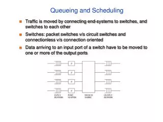
Queueing and Scheduling. Traffic is moved by connecting end-systems to switches, and switches to each other Switches: packet switches v/s circuit switches and connectionless v/s connection oriented Data arriving to an input port of a switch have to be moved to one or more of the output ports.

Queueing and Scheduling
E N D
Presentation Transcript
Queueing and Scheduling • Traffic is moved by connecting end-systems to switches, and switches to each other • Switches: packet switches v/s circuit switches and connectionless v/s connection oriented • Data arriving to an input port of a switch have to be moved to one or more of the output ports
Blocking in Packet Switches • Can have both internal and output blocking • Internal: no path to output • Output: link unavailable • Unlike a circuit switch, cannot predict if packets will block • If packet is blocked, must either buffer or drop it • Dealing with blocking: Match input rate to service rate • Overprovisioning: internal links much faster than inputs • Buffering: • input port • in the fabric • output port • shared memory • hybrid
Input Buffering (input queueing) • No speedup in buffers or trunks (unlike output queued switch) • Needs arbiter • Problem: head of line blocking
Dealing with HOL blocking • Per-output queues at inputs • Arbiter must choose one of the input ports for each output port • Parallel Iterated Matching • inputs tell arbiter which outputs they are interested in • output selects one of the inputs • some inputs may get more than one grant, others may get none • if >1 grant, input picks one at random, and tells output • losing inputs and outputs try again • Used in DEC Autonet 2 switch
Output Queueing • Don’t suffer from head-of-line blocking • Output buffers need to run much faster than trunk speed • Can reduce some of the cost by using the knockout principle • unlikely that all N inputs will have packets for the same output • Most commonly used mechanism in routers
Shared Memory • Route only the header to output port • Bottleneck is time taken to read and write multiported memory • Doesn’t scale to large switches
Scheduling • Scheduling disciplines: • resolve contention • allocate • bandwidth • delay • loss • determine the fairness of the network • give different qualities of service and performance guarantees • Components: • decides service order • manages queue of service requests • Example: consider queries awaiting web server • scheduling discipline decides service order • and also if some query should be ignored
Scheduling • Use scheduling: • Wherever contention may occur • Usually studied at network layer, at output queues of switches • Application types: • best-effort (adaptive, non-real time) • e.g. email, some types of file transfer • guaranteed service (non-adaptive, real time) • e.g. packet voice, interactive video, stock quotes • Requirements • implementation ease: few instructions or hardware • has to make a decision once every few microseconds! • work per packet should scale less than linearly with number of active connections • fairness: protection against traffic hogs • performance bounds: on bandwidth, delay and loss • admission control: needed to provide QoS
Max-Min Fairness • Scheduling discipline allocates a resource • An allocation is fair if it satisfies max-min fairness • Intuitively • each connection gets no more than what it wants • the excess, if any, is equally shared Transfer half of excess Unsatisfied demand A B A B C C
Scheduling Design Choices • Priority: • packet is served from a given priority level only if no packets exist at higher levels • highest level gets lowest delay (starvation) • Work Conservation: • conservation law: Σρiqi = constant; where ρi = λixi; λi is traffic arrival rate, xi is mean service time for packet; qi is mean waiting time at the scheduler, for connection i; • sum of mean queueing delays received by a set of multiplexed connections, weighted by their share of the link, is independent of the scheduling discipline • work conserving v/s non work conserving disciplines • Service Algorithm: • FCFS: bandwidth hogs win; no delay guarantees • service tags: arbitrarily reorder queue; provide guarantees; expensive sorting
Work Conserving v/s Non-Work-Conserving • Work conserving discipline is never idle when packets await service • Non work conserving discipline may be idle even when packets await service • main idea: delay packet till eligible • Reduces delay-jitter => fewer buffers in network • Choosing eligibility time: • rate-jitter regulator: bounds maximum outgoing rate • delay-jitter regulator: compensates for variable delay at previous hop • Always punishes a misbehaving source • Increases mean delay; Wastes bandwidth; Implementation cost
Scheduling Best-effort Connections • Main requirement is fairness • Achievable using Generalized Processor Sharing (GPS) • Visit each non-empty queue in turn • Serve infinitesimal from each • GPS is not implementable; we can serve only packets • No packet discipline can be as fair as GPS
Weighted Round Robin • Serve a packet from each non-empty queue in turn • Unfair if packets are of different length or weights are not equal • Different weights, fixed packet size • serve more than one packet per visit, after normalizing to obtain integer weights • Different weights, variable size packets • normalize weights by meanpacket size • e.g. weights {0.5, 0.75, 1.0}, mean packet sizes {50, 500, 1500} • normalize weights: {0.5/50, 0.75/500, 1.0/1500} = { 0.01, 0.0015, 0.000666}, normalize again {60, 9, 4} • problem: need to know mean packet size in advance • Used in some ATM switches
Weighted Fair Queueing (WFQ) • Deals better with variable size packets and weights • Also known as packet-by-packet GPS (PGPS) • Find finish time of a packet, had we been doing GPS; serve packets in order of their finish times • WFQ details: • Suppose, in each round, the server served one bit from each active connection • Round number is the number of rounds already completed • can be fractional • If a packet of length p arrives to an empty queue when the round number is R, it will complete service when the round number is R + p => finish number is R + p • independent of the number of other connections! • If a packet arrives to a non-empty queue, and the previous packet has a finish number of f, then the packet’s finish number is f+p • Serve packets in order of finish numbers • Finish time of a packet is not the same as the finish number
WFQ continued • A queue may need to be considered non-empty even if it has no packets in it • e.g. packets of length 1 from connections A and B, on a link of speed 1 bit/sec • at time 1, packet from A served, round number = 0.5 • A has no packets in its queue, yet should be considered non-empty, because a packet arriving to it at time 1 should have finish number 1+ p • A connection is active if the last packet served from it, or in its queue, has a finish number greater than the current round number • Assuming we know the current round number R, finish number of packet of length p • if arriving to active connection = previous finish number + p • if arriving to an inactive connection = R + p
WFQ: computing the round number • Naively: round number = number of rounds of service completed so far • what if a server has not served all connections in a round? • what if new conversations join in halfway through a round? • Redefine round number as a real-valued variable that increases at a rate inversely proportional to the number of currently active connections • With this change, WFQ emulates GPS instead of bit-by-bit RR • Iterated deletion: • A sever recomputes round number on each packet arrival • At any recomputation, the number of conversations can go up at most by one, but can go down to zero, leading to change in round number • Soln: use previous count to compute round number; if this makes some conversation inactive, recompute; repeat until no conversations become inactive
WFQ Implementation • On packet arrival: • use source + destination address (or VCI) to classify it and look up finish number of last packet served (or waiting to be served) • recompute round number • compute finish number • insert in priority queue sorted by finish numbers • if no space, drop the packet with largest finish number • On service completion • select the packet with the lowest finish number • Pros: like GPS, provides fairness and protection; can obtain worst-case end-to-end delay bound • Cons: needs per-connection state; requires a priority queue • Used in most CISCO routers
Scheduling Guaranteed-Service Connections • With best-effort connections, goal is fairness • Guaranteed-service scheduling • WFQ: provides performance (end-to-end delay) guarantees • Delay-Earliest Due Date: • Earliest-due-date: packet with earliest deadline selected • Delay-EDD prescribes how to assign deadlines to packets • A source is required to send slower than its peak rate • Bandwidth at scheduler reserved at peak rate • Deadline = expected arrival time + delay bound • Delay bound is independent of bandwidth requirement • Implementation requires per-connection state and a priority queue • Rate-controlled scheduling: Regulator shapes the traffic, scheduler provides performance guarantees
Packet Dropping • Packets that cannot be served immediately are buffered • Full buffers => packet drop strategy • Packet losses happen from best-effort connections • Shouldn’t drop packets unless imperative (wasted resources) • Common strategies: • aggregation: classify packets into classes and drop packet from class with longest queue • priorities: drop lower priority packets • endpoint or regulator marks CLP bit in packets • if network has capacity, all traffic is carried, else dropped • separating priorities within a single connection is hard • early drop: drop even if space is available • drop position: drop packet from some position in the queue
Early Random Drop and RED • Early drop => drop even if space is available • signals endpoints to reduce rate • cooperative sources get lower overall delays, uncooperative sources get severe packet loss • Early random drop • drop arriving packet with fixed drop probability if queue length exceeds threshold • intuition: misbehaving sources more likely to send packets and see packet losses • Random early detection (RED) makes three improvements: • Metric is moving average of queue lengths • Packet drop probability is a function of mean queue length • Can mark packets instead of dropping them • RED improves performance of a network of cooperating TCP sources • small bursts pass through unharmed • prevents severe reaction to mild overload • allows sources to detect network state without losses • controls queue length regardless of endpoint cooperation
Drop Position • Can drop a packet from head, tail, or random position in the queue • Tail: easy; default approach • Head: harder; lets source detect loss earlier • Random: hardest; if no aggregation, hurts hogs most