Fair Queueing
Fair Queueing. First-Come-First Served (FIFO). Packets are transmitted in the order of their arrival Advantage: Very simple to implement Disadvantage: Cannot give different service to different types of connections Each flow (even with low data rate) can experience long delays.

Fair Queueing
E N D
Presentation Transcript
First-Come-First Served (FIFO) • Packets are transmitted in the order of their arrival • Advantage: • Very simple to implement • Disadvantage: • Cannot give different service to different types of connections • Each flow (even with low data rate) can experience long delays
Also called Head-of-Line (HOL) queueing: Each traffic flow belong to a class Each class has a priority One FIFO queue for each class Transmit from the highest priority queue with a backlog Advantage: Simple Disadvantage: Tends to “starve” the lower priority classes Static Priority
FIFO Fair Queueing Fair Queueing • Attempts to implement a scheduler that simultaneously serves all flows with a backlog at the same rate • Not easy to implement Fair Queuing in a packet network
Discussion of Fair Rate Allocation • See class notes
Fair Scheduling Algorithms • Fair Queueing (FQ), a.k.a as Processor Sharing (PS) Objective: Achieve fair rate allocation • Weighted Fair Queueing (WFQ), a.k.a. Generalized Processor Sharing (GPS) Objective: Achieve weighted fair rate allocation Problem: How to realize a fair rate allocation when • Traffic is transmitted in packet of variable size • Transmission of a packet cannot be interrupted
Fair Queuing in packet networks • Approach: • Take a fluid-flow view of traffic • View output link as a “pipe” with a given width • Transmitted traffic flows like a fluid through the pipe Scheduler can transmit traffic from multiple flows at the same time • Scheduler controls the “output rate” for each flow Output rates are set to satisfy “fairness” • Result is a fluid flow schedule • Approximate fluid-flow schedule by a packet-level scheduling algorithm
Fair Queuing (FQ): From fluid to packets Flow 1 (f1 = 1) 100 Kbps Flow 2 (f2 = 1) Flow 1 (arrival traffic) 1 2 4 5 3 time Flow 2 (arrival traffic) 1 2 3 4 5 6 time Service in fluid flow system time (ms) 0 10 20 30 40 50 60 70 80 Slide from Ion Stoica
Service in fluid flow system 3 4 5 1 2 1 2 3 4 5 6 time (ms) 0 10 20 30 40 50 60 70 80 Fair Queueing (FQ): From fluid to packets (complete) Flow 1 (f1 = 1) 100 Kbps Flow 2 (f2 = 1) Flow 1 (arrival traffic) 1 2 4 5 3 time Flow 2 (arrival traffic) 1 2 3 4 5 6 time
Fair Scheduling (fluid flow) 5000 5000 Flow 2 Flow 1 4000 4000 3000 3000 2000 2000 1000 1000 0 10 40 50 70 80 20 30 60 0 10 40 50 70 80 20 30 60
Fair Scheduling (fluid flow) 5000 5000 Flow 2 Flow 1 4000 4000 3000 3000 2000 2000 1000 1000 0 10 40 50 70 80 20 30 60 0 10 40 50 70 80 20 30 60
Fair Scheduling (FQ)(fluid flow view) • There are N flows • At any time t, all backlogged flows are served at the same rate of: where B(t) is the set of backlogged flows at time t C is the capacity of the link • The total rate guarantee to a flow j is:
Weighted Fair Scheduling (WFQ)(fluid flow view) • There are N flows with weights f1 , f2 , …,fN • The service given to two backlogged flows is proportional to their weights • At any time t , the rate allocated to a backlogged flow i is: where B(t) is the set of backlogged flows at time t C is the capacity of the link • The total rate guarantee to a flow is:
FQ/WFQ Scheduling for Packets(packet-level view) • Packet-level implementation of FQ and WFQ tries to emulate the fluid-flow version • Scheduling decision: Always select the packet that will finish next in the ideal fluid-flow FQ/WFQ system
Service in fluid flow system 3 4 5 1 2 1 2 3 4 5 6 time (ms) 0 10 20 30 40 50 60 70 80 WFQ scheduling (with place holder) Flow 1 (f1 = 1) 100 Kbps Flow 2 (f2 = 1) Flow 1 (arrival traffic) 1 2 4 5 3 time Flow 2 (arrival traffic) 1 2 3 4 5 6 time Service in packet system time (ms) 0 10 20 30 40 50 60 70 80
Service in fluid flow system 3 4 5 1 2 1 2 3 4 5 6 time (ms) 0 10 20 30 40 50 60 70 80 WFQ scheduling (complete) Flow 1 (f1 = 1) 100 Kbps Flow 2 (f2 = 1) Flow 1 (arrival traffic) 1 2 4 5 3 time Flow 2 (arrival traffic) 1 2 3 4 5 6 time Service in packet system 1 3 2 3 4 1 2 4 5 6 5 time (ms) 0 10 20 30 40 50 60 70 80 Slide from Ion Stoica
Packet-level Implementation of WFQ Problems to deal with: • The finishing time of a packet in the fluid-flow system may depend on arrivals after a packet has been selected packet-level version of WFQ cannot be 100% accurate • Once started, packet transmission cannot be preemtped • Implementation: • When a packet arrives, it is assigned a “virtual finishing time” • This is the finishing time in the fluid flow system if the set of backlogged flows does not change after packet arrival • Orders packets in increasing order of virtual finishing times • Compute virtual finishing time with the help of a system virtual time
System Virtual Time • B(t) : the set of backlogged flows at time t • The rate allocated to a backlogged flow i at time t is or : service that a backlogged flow with weight 1 receives in GPS Rate of Rate of system virtual time
WFQ: System Virtual Time • WFQ uses a System Virtual Time which tracks the progress of GPS system • Suppose the times when the set B(t) changes are • Let Bl be the set of backlogged flows in time interval • Then we have • When fewer flows are active, virtual time moves faster
WFQ: Implementation • Virtual finish time of k-th packet from flow j • ajk is the arrival time andLkj is thesize of the k-th packet from flow j • Packets are sorted and transmitted in the order of virtual finishing times • Virtual times needs to be computed only at arrival time of packets • must keep track of the busy set Bl
WFQ Example (packet level) Flow 1 (arrival traffic) 1 2 4 5 3 time Flow 2 (arrival traffic) 1 2 3 4 5 6 time Virtual time V(t) 5000 4000 3000 2000 actualtransmissionorder 1 3 2 3 4 4 5 6 5 1 2 1000 0 10 20 30 40 50 60 70 80 time t time (ms) 0 10 40 50 70 80 20 30 60
WFQ Example (packet level) Flow 1 (arrival traffic) 1 2 4 5 3 time Flow 2 (arrival traffic) 1 2 3 4 5 6 time Virtual time V(t) 5000 4000 3000 2000 actualtransmissionorder 1 3 2 3 4 4 5 6 5 1 2 1000 0 10 20 30 40 50 60 70 80 time t time (ms) 0 10 40 50 70 80 20 30 60
Approximations of Fair Queueing • Since the packet implementation of WFQ is complex, packet switches often use approximations: • Weighted Round Robin (WRR) • Virtual Clock (VC) • Many others
Weighted Round Robin (WRR) • Simple emulation of GPS • Operates in “rounds” • Li is the average packet size of flow i • Calculate the number of packets to be served in each round: • For each flow i: xi = wi / Li • x = mini { xi } • For each flow i: packets_per_roundi = xi / x • WRR is a good approximation of GPS if • All flows are active • Over long periods of time
Virtual Clock (VC) • Emulates a system with transmissions in periodic intervals • Two state variables for each flow j: • auxVCj virtual transmission time of the flow • rj reserved rate • The variable auxVCj keeps track of hypothetical departure times. If all traffic from flow j is limited to the reserved rate, then auxVCj is the departure time of an arrival. • Upon arrival of a packet from flow j with sizeLjk at time ajk: • auxVCj = max (auxVCj , ajk) + Ljk / rj • StampauxVCj in packet header • Packet are transmitted in increasing order of virtual transmission times
2 5 0 1 3 4 6 7 8 9 10 11 10 12 11 3 8 7 6 5 4 2 9 1 Virtual clock order(with auxVCi) time Example: Virtual Clock (with place holder)C = 1 Mbps, r1=r2=r3=1/3 Mbps, L=1000 bits wall clock (ms)= 2 5 0 1 3 4 6 7 8 9 10 11 r1=1/3 auxVC1 time r2=1/3 auxVC2 1 2 3 4 5 6 7 8 9 10 11 12 time r3=1/3 auxVC3 1 2 3 4 time
2 5 0 1 3 4 6 7 8 9 10 11 10 11 12 2 1 8 7 9 5 6 4 3 Example: Virtual Clock C = 1 Mbps, r1=r2=r3=1/3 Mbps, L=1000 bits wall clock (ms)= r1=1/3 auxVC1= time 3 6 9 12 15 18 r2=1/3 auxVC2 = 1 2 3 4 5 6 7 8 9 10 11 12 time 3 6 9 12 15 18 r3=1/3 auxVC3 = 1 2 3 4 time 3 6 9 12 2 2 1 1 1 2 3 3 3 4 4 4 Virtual clock order(with auxVCi) time 3 3 3 6 6 6 9 9 9 12 12 12
2 5 0 1 3 4 6 7 8 9 10 11 1 2 3 4 1 2 3 4 Example: Virtual Clock (with place holder)C = 1 Mbps, r1=r2=r3=1/3 Mbps, L=1000 bits • “auxVCj = max (auxVCj , ajk) + Ljk / rj” prevents credit accumulation of idle flows wall clock (ms)= r1=1/3 auxVC1 time r2=1/3 auxVC2 1 2 3 4 time r3=1/3 auxVC3 time Virtual clock order(with auxVCi) time
2 5 0 1 3 4 6 7 8 9 10 11 3 4 1 2 1 2 3 4 Example: Virtual Clock (complete)C = 1 Mbps, r1=r2=r3=1/3 Mbps, L=1000 bits • “auxVCj = max (auxVCj , ajk) + Ljk / rj” prevents credit accumulation of idle flows wall clock (ms)= r1=1/3 auxVC1 time 3 6 9 12 r2=1/3 auxVC2 1 2 3 4 time 3 6 9 12 r3=1/3 auxVC3 time 9 12 15 18 Virtual clock order(with auxVCi) 1 1 2 2 1 3 3 2 4 4 3 4 time 3 3 6 6 9 9 9 12 12 12 15 18
Problem with Virtual Clock (with place holder) Flow that gets more than reserved rate may be penalized in the future 2 5 0 1 3 4 6 7 8 9 10 11 5 6 7 8 1 2 4 3 9 10 11 r1=1/3 auxVC1= time 3 6 9 12 15 18 21 24 r2=1/3 auxVC2 = 1 2 3 4 time 8 11 14 17 r3=1/3 auxVC3 = 1 2 3 4 time 8 11 14 17 Virtual clock order(with auxVCi) time
Problem with Virtual Clock (with place holder) Flow that gets more than reserved rate may be penalized in the future 2 5 0 1 3 4 6 7 8 9 10 11 2 1 8 3 6 5 4 7 r1=1/3 auxVC1= time 3 6 9 12 15 18 21 24 r2=1/3 auxVC2 = 1 2 3 4 time 8 11 14 17 r3=1/3 auxVC3 = 1 2 3 4 time 8 1 14 17 4 6 7 8 1 2 3 4 5 1 1 2 2 3 3 4 Virtual clock order(with auxVCi) time 3 6 9 12 15 8 8 11 11 14 14 17 17 18 21 24 time
Problem with Virtual Clock (complete) Flow that gets more than reserved rate may be penalized in the future wall clock (ms)= 2 5 0 1 3 4 6 7 8 9 10 11