Queueing Theory
Queueing Theory. Dr. Ron Lembke Operations Management. Queues. In England, they don’t ‘wait in line,’ they ‘wait on queue.’ So the study of lines is called queueing theory. Cost-Effectiveness. How much money do we lose from people waiting in line for the copy machine?


Queueing Theory
E N D
Presentation Transcript
Queueing Theory Dr. Ron Lembke Operations Management
Queues • In England, they don’t ‘wait in line,’ they ‘wait on queue.’ • So the study of lines is called queueing theory.
Cost-Effectiveness • How much money do we lose from people waiting in line for the copy machine? • Would that justify a new machine? • How much money do we lose from bailing out (balking)?
We are the problem • Customers arrive randomly. • Time between arrivals is called the “interarrival time” • Interarrival times often have the “memoryless property”: • On average, interarrival time is 60 sec. • the last person came in 30 sec. ago, expected time until next person: 60 sec. • 5 minutes since last person: still 60 sec. • Variability in flow means excess capacity is needed
Memoryless Property • Interarrival time = time between arrivals • Memoryless property means it doesn’t matter how long you’ve been waiting. • If average wait is 5 min, and you’ve been there 10 min, expected time until bus comes = 5 min • Exponential Distribution • Probability time is t =
Poisson Distribution • Assumes interarrival times are exponential • Tells the probability of a given number of arrivals during some time period T.
Ce n'est pas les petits poissons. Les poissons Les poissons How I love les poissons Love to chop And to serve little fish First I cut off their heads Then I pull out the bones Ah mais oui Ca c'est toujours delish Les poissons Les poissons Hee hee hee Hah hah hah With the cleaver I hack them in two I pull out what's inside And I serve it up fried God, I love little fishes Don't you?
Simeon Denis Poisson • "Researches on the probability of criminal and civil verdicts" 1837 • looked at the form of the binomial distribution when the number of trials was large. • He derived the cumulative Poisson distribution as the limiting case of the binomial when the chance of success tend to zero.
Binomial Distribution • The binomial distribution tells us the probability of having • x successes in • n trials, where • p is the probability of success in any given attempt.
Binomial Distribution • The probability of getting 8 tails in 10 coin flips is:
POISSON(x,mean,cumulative) • X is the number of events. • Mean is the expected numeric value. • Cumulative is a logical value that determines the form of the probability distribution returned. If cumulative is TRUE, POISSON returns the cumulative Poisson probability that the number of random events occurring will be between zero and x inclusive; if FALSE, it returns the Poisson probability mass function that the number of events occurring will be exactly x.
Queueing Theory Equations • Memoryless Assumptions: • Exponential arrival rate = = 10 • Avg. interarrival time = 1/ • = 1/10 hr or 60* 1/10 = 6 min • Exponential service rate = = 12 • Avg service time = 1/ = 1/12 • Utilization = = / • 10/12 = 5/6 = 0.833
Avg. # in System • Lq= avg # in line = • Ls = avg # in system = • Prob. n in system = • Because • We can also write it as
Example • Customers arrive at your service desk at a rate of 20 per hour, you can help 35 per hr. • What % of the time are you busy? • How many people are in the line on average? • How many people are there, in total on avg? • What are the odds you have 3 or more people there?
Queueing Example • λ=20, μ=35 so ρ=20/35 = 0.571 • Lq= avg # in line = • Ls = avg # in system = Lq+ ρ • = 0.762 + 0.571 = 1.332
Prob. Given # in System • Prob. n people in system, ρ = 0.571 • Prob 0-3 people = • 0.429 + 0.245 + 0.140 + 0.080 = 0.894 • Prob 4 or more = 1-0.894 = 0.106
Average Time • Wq = avg wait in line • Ws = avg time in system
How Long is the Wait? • Time waiting for service = • Lq = 0.762, λ=20 • Wq = 0.762 / 20 = 0.0381 hours • Wq = 0.0381 * 60 = 2.29 min • Total time in system = • Ls = 1.332, λ=20 • Ws = 1.332 / 20 = 0.0666 hours • Ws = 0.0666 * 60 = 3.996 = 4 min • μ=35, service time = 1/35 hrs = 1.714 min • Ws = 2.29 + 1.71 = 4.0 min
What did we learn? • Memoryless property means exponential distribution, Poisson arrivals • Results hold for simple systems: one line, one server • Average length of time in line, and system • Average number of people in line and in system • Probability of n people in the system