Advanced Plotting Techniques
Advanced Plotting Techniques. Chapter 11. Above: Principal contraction rates calculated from GPS velocities. Visualized using MATLAB. Advanced Plotting. We have used MATLAB to visualize data a lot in this course, but we have only scratched the surface…

Advanced Plotting Techniques
E N D
Presentation Transcript
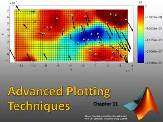
Advanced Plotting Techniques Chapter 11 Above: Principal contraction rates calculated from GPS velocities. Visualized using MATLAB.
Advanced Plotting We have used MATLAB to visualize data a lot in this course, but we have only scratched the surface… • Mainly used ‘plot’, ‘plot3’, ‘image’, and ‘imagesc’ • This section will cover some of the more advanced types of visualizations that MATLAB can produce • Vector plots • Streamline plots • Contour plots • Visualizing 3D surfaces • Making animations (if there is time) • In general, if you can picture it, MATLAB can probably do it • If not, visit MATLAB central, and it is likely that someone has written a script/function to do what you want http://www.mathworks.com/matlabcentral/fileexchange/
Vector Plots • Plotting vectors is very useful in Earth sciences • Wind velocities • Stream flow velocities • Surface velocities or displacements • Glacier movements • Ocean currents • …and many more! • Conventions: • Spatial coordinates: [x, y, z] • I.e. the location of the tail of the vector • Vector magnitudes: [u, v, w] • I.e. the [east, north, up] components of the vector MATLAB typically needs to know: In 2D: x, y, u, v In 3D: x, y, z, u, v, w [u, v] = [2.50, 4.33] 60° [x, y] = [2, 3]
Quiver Plots MATLAB provides several built-in commands for plotting vectors • I will only cover ‘quiver’ and ‘quiver3’ Keys to success: • x, y, u, and v must all be the same dimensions • Can accept vectors or matrices • WARNING! Quiver automatically scales vectors so that they do not overlap • The actual visualized vector length is not at the same scale as x/y axes
Quiver Options • quiver has lots of options • The plot shown here is silly • Made only to demonstrate some options • For list of all options >> doc quivergroup
Quiver3: 3D Vectors • ‘quiver3’ works just like ‘quiver’ except that three locations [x,y,z], and three vector components [u,v,w] are required • Uses same “quivergroup” properties
Streamline Plots • streamline: predicts & plots the path of a particle that starts within the data range • Requires a vector field • I.e. locations of many vectors and the vector magnitudes/directions • Useful for tracking contaminants, and lots more • Will not extrapolate • Works with 2D or 3D data
Calculating Particle Paths: stream2 • stream2: calculates particle paths given a velocity field • Requires x,y,u, and v • Output is a cell. [x,y] vals are in columns in the cell • For 3D paths, see stream3 Sometimes you only want the [x,y] path E.g. you may want to plot on a map projection
Streamline Plot: Example 2 • Recall that streamline does not extrapolate
Visualizing 3D Data MATLAB provides several built-in visualization functions to display 3D data • 2D Plots of 3D Data: • Contour Plots ‘contour’ • Contour Filled Plots ‘contourf’ • 3D Plots of 3D Data: • 3D Surfaces ‘surf’ ‘trisurf’ • Most of these functions require gridded data • We will cover 2D/3D interpolation and gridding
Some Useful Options for 3D Plotting Let’s contour this equation using MATLAB!
Contour Plotting Gridded Data • If your data is already regularly gridded in meshgrid format, contouring is easy… • Are these both positive peaks, or negative, or a combination? • Need to either: • Label contours with text • Draw contours using a colormap
Labeling Contours • contour can label contours • C contains contour info • h is the handle to the contour group • Often the labels are at awkward intervals • How can I specify which contours to plot?
Specifying Contour Labels • Contour labeling is very flexible and customizable • For more information and settings read the documentation >> doc contour >> doc clabel
Coloring Contours Using a Colormap • If no color is specified, MATLAB uses the default colormap, jet, to color the contour lines • Use colorbar to display the colorbar • How can I specify the colormap and the colormap limits?
Coloring Contours Using a Colormap • Color maps and ranges can be specified! • How can make a color filled contour plot? • Dr. Marshall’s favorite!
Filled Contour Plots • contourfmakes color-filled contour plots • Can specify the colormap and caxis range if needed
Filled Contour Plots: Some Options • Color-filled contour plots are an excellent way to visualize 3D data in a 2D format • If color is not an option, use colormap(gray)
3D Mesh Plot • Makes a rectangular mesh of 3D data • Unless color is specified, mesh is colored by a colormap
3D Surface Plots • Surface plots use solid colored quadrilaterals to make a 3D surface • Num of elements depends on [x,y] spacing
Gridding/Interpolating 3D Data • All of the previously discussed, 3D data visualization commands require data on a regular grid • What if your data is unevenly spaced or scattered? • You must first grid the data (interpolate it) • MATLAB provides a few really nice tools for this task • I will only cover: griddata & scatteredinterpolant
Let’s Make a Scattered Data Set For all the forthcoming examples, we need scattered data • Let’s make two scattered data sets of [x, y] to be loaded • A simple plain: • The same exponential function as before:
Convex Hulls & Extrapolation When calling some gridding/interpolating functions in MATLAB, extrapolation is not performed by default • What is extrapolation in 2D/3D? • Any point that falls outside of the convex hull is typically considered to be extrapolated • Convex hull: An outline of your data’s limits • convhull: returns the indices of the input [x,y] values that are at the outer edges of the data range
Gridding Non-Uniform Data: griddata griddata interpolates z-values from non-uniform (or uniform) data Requires: • scattered [x,y,z] *(can also interpolate gridded [x,y,z] data) • new grid data points [x,y] (from meshgrid)
griddata: Interpolation Methods griddata offers several interpolation methods Which is best? No straightforward answer Depends on your data and sampling If you don’t know, stick with linear (default)
Other Ways to Interpolate 2D/3D Data • interp2 / interp3: will also interpolate a 2D/3D dataset, but the scattered data must be monotonically increasing. • I.e. the data must follow a constant and predictable direction • Doesn’t do anything that griddata or scatteredInterpolant doesn’t already do • While griddata works fine for most applications, it is not highly optimized • So, if your data set is huge, consider using scatteredInterpolant • scatteredInterpolant: Accepts [x, y, z] data and returns a function that can be used to interpolate/extrapolate the data at any user-specified value • Advantages: Faster than griddata. More reliable interpolation algorithm • Disadvantages: Requires a bit more coding than griddata. Will extrapolate by default. Only in MATLAB 2013a or newer
scatteredInterpolantExample 1 • Interpolate the scattered planar data Warning!! scatteredInterpolant extrapolates by default!
scatteredInterpolantExample 2 • Interpolate the scattered exponential data What interpolation options are there for scatteredInterpolant?
scatteredInterpolant: Interpolation Methods scatteredInterpolant has three interpolation methods See documentation for usage Also has two extrapolation methods Or you can turn extrapolation off Now that you know how to grid/interpolate scattered data you can make any of the 3D plots shown earlier!
Triangulation • What if you have scattered data that you do not want to interpolate? • Typically, you will triangulate the data and make the data into a triangulated surface • Determining the optimal triangulation is non-trivial, but MATLAB has a built-in function that calculates the optimal triangulation, delaunay • Called a Delaunay triangulation
3D Triangulated Surfaces: trisurf 'FaceColor','interp'
Comparison: surf vs. trisurf 'FaceColor','interp' 'FaceColor','interp'
Final Thoughts • MATLAB is a powerful tool for processing quantitative data • MATLAB is not the only tool for data analysis • Is not ideal for all analyses, but is very good for most • Not all Earth scientists know how to code…but they should! • Knowing how to write your own code gives you the freedom to create customized tools • Tools that save time • Reduce errors from repetitive tasks • Avoid re-doing data analyses multiple times • Coding allows you to develop new research methods • Don’t need to wait for a program to have a button. You can be the one that makes the buttons • Although you now know that buttons are inefficient