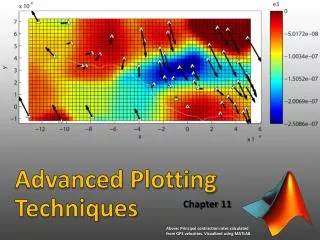
Advanced Plots in MATLAB: Leveraging FPLOT, Logarithmic & Polar Charts
This guide explores advanced plotting techniques in MATLAB, focusing on the FPLOT function to visualize functions defined as strings, and utilizing logarithmic scales for better viewing of exponential functions. It covers various chart types including SEMILOGX, SEMILOGY, LOGLOG, and POLAR plots with practical examples. Learn how to create dynamic plots with animated comet charts and manage multiple plots in one window using the SUBPLOT command for effective data visualization.

Advanced Plots in MATLAB: Leveraging FPLOT, Logarithmic & Polar Charts
E N D
Presentation Transcript
FPLOT • Plots a function f(x) written as a string within quotation marks. The free variable needs to be designated with x. • The lower and upper limits for x are given as a row vector with two values, as the second argument of the function. • Example: fplot('x.*sin(x)', [0 10*pi])
FPLOT example • Example of fplot:fplot('x.*sin(x)', [0 10*pi])
Logarithmic plotting • Many functions tend to increase exponentially after some point. This presents problems in viewing the behavior (or see the values) of the function where it is close to zero. • To accentuate low values and compress the high ones, the axis where the values get too high are plotted on a logarithmic scale. • In MATLAB, we can plot x-axis, y-axis, or both axes on a logarithmic scale.
Chart type: SEMILOGX • Example:x= e-t, y= t, 0≤t≤2 t= linspace(0, 2*pi, 200);x= exp(-t); y= t;plot(x,y); grid; t= linspace(0, 2*pi, 200);x= exp(-t); y= t;semilogx(x,y); grid;
Chart type: SEMILOGY • Example:y= e-x2, -3 ≤ x ≤ 3 x= linspace(-3, 3, 101);y= exp(-x.^2);plot(x,y); grid; x= linspace(-3, 3, 101);y= exp(-x.^2);semilogy(x,y); grid;
Chart type: LOGLOG • Example:x= e-t, y= 100 + e2t, 0 ≤ t ≤ 2 t= linspace(0, 2*pi, 200);x= exp(-t); y= 100+exp(2*t);plot(x,y); grid; t= linspace(0, 2*pi, 200);x= exp(-t); y= 100+exp(2*t);loglog(x,y); grid;
Chart type: POLAR • Plots a radial function around 360° • Example:r2= 2 sin 5t, 0 ≤ t ≤ 2t= linspace(0, 2*pi, 200);r= sqrt(abs(2*sin(5*t)));polar(t,r);
Chart type: FILL • Example:r2= 2 sin 5t, 0 ≤ t ≤ 2x= r cos t, y= r sin tt= linspace(0, 2*pi, 200);r= sqrt(abs(2*sin(5*t)));x= r.*cos(t); y= r.*sin(t);fill(x,y,'r');axis('square');
Chart type: BAR • Example:r2= 2 sin 5t, 0 ≤ t ≤ 2y= r sin tt= linspace(0, 2*pi, 200);r= sqrt(abs(2*sin(5*t)));y= r.*sin(t);bar(t,y);axis([0 pi 0 inf]);
Chart type: BARH • Example: World population by continentscont= char('Asia', 'Europe', 'Africa', 'N.America', 'S.America');pop=[3332; 696; 694; 437; 307];barh(pop);for i=1:5 gtext(cont(i,:));endxlabel('Population in millions');title('World population 1992');
Chart type: PIE • Example: World population by continentscont= char('Asia', 'Europe', 'Africa', 'N.America', 'S.America');pop=[3332; 696; 694; 437; 307];pie(pop);for i=1:5 gtext(cont(i,:));endtitle('World population 1992');
Chart type: COMET • Animated linear plot. Example: b= a sin a, 0 ≤ a ≤ 10a= linspace(0, 10*pi, 2000); b= a.*sin(a); pause(2); comet(a, b);
Multiple charts in a window • Multiple plots may be placed in a window using the SUBPLOT command. • Syntax: subplot(rows, columns, active) • Any plotting command acts on the active subplot only. • Active plot is selected in row-major order.
Multiple charts in a window • Example:x= linspace(0, 4*pi, 100); subplot(3,2,1); plot(x, sin(x));subplot(3,2,2); plot(2*x, sin(2*x));subplot(3,2,3); plot(x, cos(x));subplot(3,2,4); plot(2*x, cos(2*x));subplot(3,2,5); plot(x, tan(x));subplot(3,2,6); plot(2*x, tan(2*x));