Plotting
Plotting. Overview plot in 2D Plot in 3D Other possible charts Engineers: label your plots! Plots & Polynomial. 1. 1. Plots & Charts, overview. Plotting functions plot(), plot3(), polar(), meshgrid() Charting functions pie(), pie3(), bar(), bar3(), bar3h(), hist(), errorbar()


Plotting
E N D
Presentation Transcript
Plotting Overview plot in 2D Plot in 3D Other possible charts Engineers: label your plots! Plots & Polynomial 1
1. Plots & Charts, overview • Plotting functions plot(), plot3(), polar(), meshgrid() • Charting functions pie(), pie3(), bar(), bar3(), bar3h(), hist(), errorbar() • Plot-related functions polyfit(), polyval(), text(), title(), xlabel(), ylabel() 2
2. Plots • Create a graph of y vs. x plot(x, y) %order of arguments matters • Example: 100 data-points x = linspace(-pi, pi); y = sin(x); plot(x, y) • By default, plot()connects the data-points with a solid line without markers. 3
2. Plots, cont. • Let us try with less data-points: x = linspace(-pi, pi, 10); y = sin(x); plot(x, y); • Notice that the curve is less smooth • This is another reason why linspace() is friendly to use: easily fixable. 4
2. Plots: line specifiers • A third argument can be added in the plot function-call: plot(x,y, _____) • The third argument must be a string, made of up to three components: • One component for the line’s color • One component for the line-style • And one component for the marker symbol (the symbol at each data point 5
2. Plots: lineSpecs - color • Specify the color only: plot(x, y, ‘r’); 6
2. Plots: lineSpecs – line style • Colorand line-style: plot(x, y, ‘r:’); (none): no line 7
2. Plots: lineSpecs - marker • Color, type of line and data-marker: plot(x, y, ‘r:d’); 8
2. Plots: line specifier, cont. • If only the data-points must show, leave out the line-style: plot(x, y, 'rd') • Forgot all the options? >> doc plot <enter> 9
2. Plots: multiple plots • Repeat the series of 3 arguments to combine multiple plots on 1 graph. • Example: X = linspace(-2*pi,2*pi,50); Ysine = sin(X); Ycosine = cos(X); plot(X,Ysine,'r:o',X,Ycosine,'b--d') • The string argument is unnecessary. MATLAB will rotate through the default colors to make sure each plot has a different color. The other 4 arguments are MANDATORY.
2. Plots: hold on/off • At default mode, the plot() command erases the previous plots before drawing new plots. • If subsequent plots are meant to add to the existing graph, use: hold on, which holds the current plot. • When you are done, use hold off to return to default mode. • hold, by itself, toggles the hold modes.
2. Plots: hold on/off, cont. >> x1 = linspace(0,pi,25); >> plot(x1,sin(x1),'r') >> hold on >> plot(x1,sin(2*x1),'g’) * Range of the axis will be automatically adjusted.
3. Plots: 3 dimensions • plot3() makes a 3D plot – requires x, y, and z data. 13
Meshgrid() Given: x = [1 2 3]; y = [4 5]; Evaluate: f(x,y) = x + y In other words, I need to evaluate (x+y) at every pair of points between x and y.
Meshgrid(), cont. To make a useful plot, it is necessary to match up each x with each y before computing z. The function meshgrid() makes this easy to do. 15
3. Plots: 3 dimensions, cont. x = linspace(-pi, pi); y = linspace(-pi, pi); [X, Y] = meshgrid(x, y); Z = sin(X).^3 - cos(Y).^2; plot3(X, Y, Z) Creates two arrays X, Y where each value of x is matched with each value of y 16
4. Other Possible Charts • polar() creates polar coordinate plots: x = linspace(-pi, pi); y = cos(x) - sin(x).^2; polar(x, y) 17
4. Other Possible Charts, cont. • pie(), pie3(), bar(), bar3(), bar3h(), hist(), errorbar() pie3() >> x = 38 54 8 54 48 >> pie3(x) Much like Excel offers: 18
4. Other Possible Charts, cont. • pie(), pie3(), bar(), bar3(), bar3h(), hist(), errorbar() bar3h() x = 8 9 1 9 6 >> bar3h(x) Much like Excel offers: 19
4. Other Possible Charts, cont. • pie(), pie3(), bar(), bar3(), bar3h(), hist(), errorbar() errorbar() 20
4. Other Possible Charts, cont. • As with all the MATLAB possibilities, use… F1 = Help 21
5. Engineers: Complete Plots • The following built-in functions should be applied to any graph created: title() %title on figure xlabel() %x-axis label ylabel() %y-axis label zlabel() %z-axis label • Each function takes 1 ‘string’ argument only and has no return-value. 22
5. Engineers: Complete Plots • Additional built-in function: text() Example: text(1, -2, -2, 'Cool plot!') 23
5. Engineers: Complete Plots • Built-in function: grid on COMMAND line typed in the script, after a plot command. • It stands alone on one line, requires no arguments, and returns no value. 24
5. Engineers: Complete Plots • Additional built-in functions: legend(), xlim, ylim,… 25
6. Plotting & Polynomials • Plot-related functions that try to find an equation that links data-points: polyfit(), polyval() • polyfit() is like linear regression which finds the curve that best fits the data-points. polyfit() attempts to fit a polynomial – not a line. It mainly finds the coefficients of the polynomial that best fits the data given. • polyval() is used to evaluate the polynomial at specified points. It makes use of the coefficients generated by polyfit(). • It is frequently used to generate a plot. 26
6. Plotting & Polynomials, cont. clear clc %generate tables of x, and y data = [1, 50; 4, 4900; 7, 4600; 10, 3800; 70, 1300; 100, 850; 300, 0.2e9; 700, 1.2e9; 1000, 1.2e9]; x = data(:, 1)'; y = data(:, 2)'; %plot data points, omit line plot(x, y, 'd') hold on %combine future plots on this one %find best-fit polyn. of order 3 coeff= polyfit(x, y, 3) px = linspace(min(x), max(x), 100); py = polyval(coeff, px); plot(px, py) Remember that fitting a curve does NOT mean hitting every data-point! 27
Wrapping Up • Plotting any kind of graphs mostly requires vectors of identical dimensions: (x,y) (x, y, z) (r, theta, z)... • hold on allows multiple plots to be combined together. • The independent variable is the first argument. IT IS A COMMON MISTAKE TO SWAP THEM. • All functions are easily explained in the help, usually with examples that show how to place arguments. • As engineer, remember all graphs must be labeled correctly. • For mathematical analysis, polyfit() and polyval() allow to fit a curve through data-points. 28