Plotting
Plotting. ELEC 206 Computer Applications for Electrical Engineers Dr. Ron Hayne. Two-Dimensional Plots. x-y Plot x-axis independent variable y-axis dependent variable x = [1:10]; y = [58.5, 63.6, 64.2, 67.3, 71.5, ... 88.3, 90.1, 90.6, 89.5, 90.4]; plot(x,y). Basic Plotting.

Plotting
E N D
Presentation Transcript
Plotting ELEC 206 Computer Applications for Electrical Engineers Dr. Ron Hayne
Two-Dimensional Plots • x-y Plot • x-axis • independent variable • y-axis • dependent variable x = [1:10]; y = [58.5, 63.6, 64.2, 67.3, 71.5, ... 88.3, 90.1, 90.6, 89.5, 90.4]; plot(x,y) 206_M4
Basic Plotting • Labels plot(x,y) title('Lab 1') xlabel('Voltage') ylabel('Current') grid on plot(x,y), title('Lab 1'), xlabel('Voltage'), ylabel('Current'), grid on 206_M4
Basic Plotting • Figure Control • pause, pause(n) • figure, figure(n) • Multiple Plots • hold on, hold off • plot(X, Y, W, Z) • plotyy(X, Y, W, Z) • Subplots • subplot(m,n,p) • m-by-n grid • pth window 206_M4
Basic Plotting • Style Control • Axis Scaling • axis, axis(v) • v = [xmin,xmax,ymin,ymax] • Annotation • legend('string1', 'string2') 206_M4
Example figure(3) x = 0:pi/100:2*pi; y1 = cos(4*x); y2 = sin(x); plot(x,y1,':r',x,y2,'--b') 206_M4
Other Plots • Polar Plots • polar(theta,rho) • Example figure(4) polar(x,y1,':r') hold on polar(x,y2,'--b') 206_M4
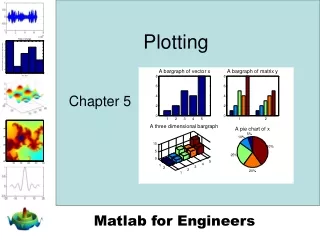
Other Plots • Logarithmic Plots • semilogx(x,y) • semilogy(x,y) • loglog(x,y) • Bar Graphs and Pie Charts • bar(x), barh(x) • bar3(x), bar3h(x) • pie(x), pie3(x) • Histograms • hist(x), hist(x,bins) 206_M4
Problem Solving Applied • UDF Engine Performance • Problem Statement • Calculate the velocity and acceleration using a script M-file • Input/Output Description Start Time = 0 sec Velocity Final Time = 120 sec Acceleration Time Increment = 10 sec 206_M4
Problem Solving Applied • Hand Example • velocity = 0.00001 time3 - 0.00488 time2 + 0.75795 time + 181.3566 • acceleration = 3 - 0.000062 velocity2 • For time = 100 sec • velocity = 218.35 m/sec • acceleration = 0.04404 m/sec2 • Algorithm Development (outline) • Define time matrix • Calculate velocity and acceleration • Output results in table 206_M4
MATLAB Solution clear, clc %Example 4.3 %These commands generate velocity and acceleration %values for a UDF aircraft test %Define the time matrix time = 0:10:120; %Calculate the velocity matrix velocity = 0.00001*time.^3 - 0.00488*time.^2 ... + 0.75795*time + 181.3566; %Use calculated velocities to find the acceleration acceleration = 3 - 6.2e-5*velocity.^2; %Present the results in a table [time', velocity', acceleration'] 206_M4
Table Output 206_M4
Plotting Results %Create x-y plots plot(time,velocity) title('Velocity of a UDF Aircraft') xlabel('time, seconds') ylabel('velocity, meters/sec') grid on % figure(2) plot(time, acceleration,':k') title('Acceleration of a UDF Aircraft') xlabel('time, seconds') ylabel('acceleration, meters/sec^2') grid on 206_M4
Plotting Results %Use plotyy to create a scale on each side of plot figure(3) plotyy(time, velocity,time,acceleration) title('UDF Aircraft Performance') xlabel('time, seconds') ylabel('velocity, meters/sec') grid on 206_M4
Three-Dimensional Plotting • 3-D Line Plot • plot3(x,y,z) • Surface Plots • mesh(z), mesh(x,y,z) • surf(z), mesh(x,y,z) • shading, colormap • Contour Plots • contour(z), contour(x,y,z) • surfc(z), surfc(x,y,z) 206_M4
Example figure(5) z=peaks(25); surfc(z) colormap(jet) 206_M4
More Plotting • Creating Plots from the Workspace Window • Plotting Icon • Editing Plots from the Menu Bar • Copy Figure 206_M4
Summary • Two-Dimensional Plots • Problem Solving Applied • Three-Dimensional Plots • End of Chapter Summary • MATLAB Summary • Characters, Commands and Functions 206_M4
Test #3 Review • MATLAB Environment • MATLAB Windows • Scalar Operations • Array Operations • Saving Your Work • Predefined MATLAB Functions • MATLAB Functions • Manipulating Matrices • Special Values and Functions 206_M4
Test #3 Review • Plotting • Two-Dimensional Plots • Three-Dimensional Plots • Applications • Data Analysis 206_M4