Graph Plotting:
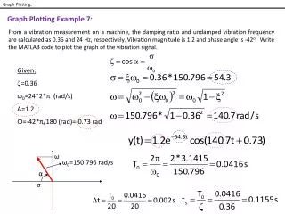
Graph Plotting:. Given: z =0.36 ω 0 =24*2* π (rad/s) A=1.2 Φ =-42* π /180 (rad)=-0.73 rad. ω. ω 0 =150.796 rad/s. α. - σ. Graph Plotting Example 7:.

Graph Plotting:
E N D
Presentation Transcript
Graph Plotting: Given: z=0.36 ω0=24*2*π (rad/s) A=1.2 Φ=-42*π/180 (rad)=-0.73 rad ω ω0=150.796 rad/s α -σ Graph Plotting Example 7: From a vibration measurement on a machine, the damping ratio and undamped vibration frequency are calculated as 0.36 and 24 Hz, respectively. Vibration magnitude is 1.2 and phase angle is -42o. Write the MATLAB code to plot the graph of the vibration signal.
Graph Plotting: clc;clear t=0:0.002:0.1155; yt=1.2*exp(-54.3*t).*cos(140.7*t+0.73); plot(t,yt) xlabel(‘Time (s)'); ylabel(‘Displacement (mm)'); Displacement (mm) Time (s)
Roots of a polynomial: Find the roots of the polynomial. with Matlab >> p=[3 0 5 6 -20] >> roots(p) >>ezplot('3*t^4+5*t^2+6*t-20',-2,2) ans = -1.5495 0.1829 + 1.8977i 0.1829 - 1.8977i 1.1838
Solution of nonlinear equations: Newton-Raphson Example: The time-dependent locations of two cars denoted by A and B are given as At which time t, two cars meet?
Solutions of system of nonlinear equations: Alternative Solutions with MATLAB clc;clear t=solve('t^3-t^2-4*t+3=0'); vpa(t,6) Newton-Raphson Example: clc, clear x=1;xe=0.001*x; niter=20; %---------------------------------------------- for n=1:niter %---------------------------------------------- f=x^3-x^2-4*x+3; df=3*x^2-2*x-4; %---------------------------------------------- x1=x x=x1-f/df if abs(x-x1)<xe kerr=0;break end end kerr,x Using roots command in MATLAB a=[ 1 -1 -4 3]; roots(a) ANSWER t=0.713 s t=2.198 s
Solution of system of nonlinear equations: How do you find x and y values, which satisfy the equations? with Matlab: >>[x,y]=solve('sin(2*x)+y^3=3*x-1','x^2+y=1-y^2') x=0.6786, y=0.3885 clc, clear x=[1 1]; xe=[0.01 0.01]; niter1= 5; niter2=50; fe=transpose(abs(fe));kerr=1; for n=1:niter2 x %-----Error equations------------------------ a(1,1)=2*cos(2*x(1))-3;a(1,2)=3*x(2)^2; a(2,1)=2*x(1);a(2,2)=2*x(2)+1; b(1)=-(sin(2*x(1))+x(2)^3-3*x(1)+1); b(2)=-(x(1)^2+x(2)^2+x(2)-1); %------------------------------------------------------- bb=transpose(b);eps=inv(a)*bb;x=x+transpose(eps); if n>niter1 if abs(eps)<xe kerr=0; break else display ('Roots are not found') end end end x=0.6786 y=0.3885
Solution of system of nonlinear equations: How do you calculate a and b, which satisfy given equations by computer? clc, clear x=[1 1]; xe=[0.01 0.01]; niter1= 5; niter2=50; fe=transpose(abs(fe));kerr=1; for n=1:niter2 x %-----Error equations------------------------ a(1,1)=6*x(1);a(1,2)=4*x(2); a(2,1)=6*x(1)^2;a(2,2)=2*(x(2)-1); b(1)=-(3*(x(1)^2-1)+2*x(2)^2-11); b(2)=-(2*x(1)^3+(x(2)-1)^2-16); %------------------------------------------------------- bb=transpose(b);eps=inv(a)*bb;x=x+transpose(eps); if n>niter1 if abs(eps)<xe kerr=0; break else display ('Roots are not found') end end end With Matlab >>[a,b]=solve('3*(a^2-1)+2*b^2=11','2*a^3+(b-1)^2=16') Matlab gives all possible solutions
Lagrange Interpolation: Example: The temperature (T) of a medical cement increases continuously as the solidification time (t) increases. The change in the cement temperature was measured at specific instants and the measured temperature values are given in the table. Find the cement temperature at t=36 (sec).
Lagrange Interpolation: Example: The buckling tests were performed in order to find the critical buckling loads of a clamped-pinned steel beams having different thicknesses. The critical buckling loads obtained from the experiments are given in the table. Find the critical buckling load Pcr (N) of a steel beam with 0.8 mm thickness. Pcr 0.8 mm
Lagrange Interpolation: data.txt 0.5,30 0.6,35 0.65,37 0.73,46 0.9,58 Pcr 1. Lagrange Interpolation with Matlab clc;cleart=[0.5 0.6 0.65 0.73 0.9];P=[30 35 37 46 58];interp1(t,P,0.8,'spline') 0.8 mm 2. Lagrange Interpolation with Matlab clc;clear v=load ('c:\saha\data.txt') interp1(v(:,1),v(:,2),8,'spline')
Lagrange Interpolation: • The pressure values of a fluid flowing in a pipe are given in the table for different locations . Find the pressure value for 5 m. • a) Lagrange interpolation (manually) • with computer a) with Lagrange interpolation b) For computer solution, the MATLAB code is given as clc;clearx=[3 8 10];P=[7 6.2 6];interp1(x,P,5,'spline')
Lagrange Interpolation: The x and y coordinates of three points on the screen, which were clicked by a CAD user are given in the figure. Find the y value of the curve obtained from these points at x=50. • How do you find the answer with computer? clc;clearx=[25 40 70];y=[-10 20 5];interp1(x,y,50,'spline') Result: 26.111 b) How do you find the answer manually?
Simpson’s Rule: Example: Calculate the volume of the 3 meter long beam whose cross section is given in the figure. Solution with Matlab: >>syms x; area=int((x+1)/(sqrt(x^2+4)),0,1.2);vpa(area,5) Area=0.9012
Simpson’s Rule: Calculate the integral with; a) Trapezoidal rule b) Simpson’s rule c) Using MATLAB, take n=4. a) Trapezoidal rule: Divide into for equal sections between 0.5 and 1.
Simpson’s Rule: b) Simpson’s rule: using Matlab >>syms tet >>I=int(sqrt(tet)*cos(tet),0.5,1);vpa(I,5) I=0.30796
Lagrange Interpolation + Simpson’s Rule: Example: For a steel plate weighing 10 N and has a thickness 3 mm, the the coordinates of some points shown in the figure were measured (in cm) by a Coordinate Measuring Machine (CMM). How do you calculate the intensity of the steel by fitting a curve, which passes through these points. ? a) Manual calculation: The volume of the part is calculated by using its surface area and 0.3 cm thickness value. The simpson’s rule is used for area calculation. The x axis must be divided in equal segments in this method. Since the points are not equally spaced on the x axis, the necessary y values should be calculated at suitable x values. If we divide the interval 0-4 into four equal sections using the increment ∆x=1 , we can obtain the y values for x=1, x=2 and x=3.
Lagrange Interpolation + Simpson’s Rule: b) With computer: For calculation with computer, MATLAB code is arranged to find the y values for x=1, x=2 and x=3 and the code Lagr.I is run. clc;clearx=[0 2.5 3.7 4];y=[5 7.8 9.3 10];interp1(x,y,1,'spline') interp1(x,y,2,'spline') interp1(x,y,3,'spline') The area of the plate can be calculated by using Simpson’s rule. Then, the density of the steel can be calculated as mentioned before.
Simpson’s Rule: 4.2i -1.4 Example: Calculate the integral of the given function.
Simpson’s Rule: Solution with Matlab: >>clc;clear; >> syms teta >>f=2.5*exp(-1.4*teta)*cos(4.2*teta+1.4) >>y=int(f,0,4.49) >>vpa(y,5) I=-0.4966
Simpson’s Rule: Example:
Simpson’s Rule: Solution with Matlab: >>clc;clear; >> syms teta >>f=(2.5*exp(-1.4*teta)*cos(4.2*teta+1.4))^2 >>y=int(f,0,4.49) >>vpa(y,5) I=0.898 We must increase the number of sections!
Simpson’s Rule: A stationary car starts to move with the acceleration given below • Find the speed of the car at the end of 10 seconds • Manually • With computer a) b) With computer using Matlab >>syms t >>I=int((1+sin(t)^3)/sqrt(t^2+1),0,10);vpa(I,5)
Simpson’s Rule: Roots Find the intersection area of the curves y=x2+2 ile y=3x . >> roots([1 -3 2]) using Matlab >>syms x >>I=int(3*x-x^2-2,1,2);vpa(I,5)
System of linear equations: How do you calculate u,w and z with computer? With Matlab clc;clear a=[-1 1 -3;0 3 -6;1 1 1]; b=[9;12;5]; c=inv(a)*b
System of linear equations: F b A As a result of the equilibrium conditions, the equations given below are obtained for a truss system. How do you calculate the member forces FJD, FFD, FCD and FFC if FCK=6.157 kN and FCB=-3.888 kN are known?
System of linear equations: with Matlab clc;clear A=[-1 -0.707 -0.894 0;0 -0.707 -1 0;3 0 0 2.365;0 0 0.894 1]; b=[-0.466;0;-6.557;4.353]; F=inv(A)*b FJD= 1.5429 kN FFD= -14.3701 kN FCD= 10.1596 kN FFC= -4.7297 kN F b A