Decadal Climate Variability and Predictions in the Atlantic
350 likes | 376 Vues
This workshop explores the mechanisms and predictability of decadal climate variability in the Atlantic region, and its societal relevance. It also discusses the adequacy of current models and observing systems for decadal prediction.

Decadal Climate Variability and Predictions in the Atlantic
E N D
Presentation Transcript
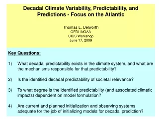
Decadal Climate Variability, Predictability, and Predictions - Focus on the AtlanticThomas L. DelworthGFDL/NOAACICS WorkshopJune 17, 2009 Key Questions: • What decadal predictability exists in the climate system, and what are the mechanisms responsible for that predictability? • Is the identified decadal predictability of societal relevance? • To what degree is the identified predictability (and associated climatic impacts) dependent on model formulation? • Are current and planned initialization and observing systems adequate for the job of initializing models for decadal prediction?
Outline • Components of decadal predictability • Climatic relevance of the Atlantic • Mechanisms of Atlantic variability • Underpinnings for decadal prediction • GFDL decadal predictability/prediction activities
Crucial points: • Robust predictions will require sound theoretical understanding of decadal-scale climate processes and phenomena. • Assessment of predictability and its climatic relevance may have significant model dependence, and thus may evolve over time (with implications for observing and initialization systems). But … even if decadal fluctuations are not predictable, it is still important to understand them to better understand and interpret observed climate change.
Components of decadal variability and predictability • Forced climate change • Predictability arising from estimates of future changes in radiative forcing agents, and the climate system response to those changes. • “Committed warming” from past radiative forcing • Internal variability • Decadal-scale fluctuations are an important part of climate variability • Is there “meaningful” decadal-scale predictability in the climate system? • Can we realize that predictability? • Is the “natural” variability altered by radiative forcing?
North Atlantic Temperature Why look to the Atlantic for decadal predictability? What will the next decade or two bring? Warm North Atlantic linked to … Drought More rain over Sahel and western India More intense hurricanes • Two important aspects: • Decadal-multidecadal fluctuations • Long-term trend
Impacts of Atlantic Multidecadal Variability SLP Rainfall Air Temperature Simulated atmospheric response to imposed SST anomalies in the Atlantic using the Hadley Centre atmospheric model (HADAM3). Aug-Oct. Sutton and Hodson, 2005.
JJA Precipitation Anomalies Associated with Maximum MOC Paleo and modern records show global scale impact of Atlantic SST anomalies on rainfall, SST, and circulation. Units: cm/day
Projected Atlantic SST Change (relative to 1991-2004 mean) Can we predict which trajectory the real climate system will follow? Results from GFDL CM2.1 Global Climate Model
What is the mechanism behind Atlantic multidecadal variability? Two different, but not mutually exclusive, ideas: • Atlantic Multidecadal Variability is a product of internal variability of the climate system through multidecadal scale strengthening and weakening of the Atlantic Meridional Overturning Circulation (AMOC). • Atlantic Multidecadal Variability is a product of changing radiative forcing (greenhouse gases and aerosols) in the 20th century.
“Comparing the results to observations, it is argued that the long-term, observed, North Atlantic basin-averaged SSTs combine a forced global warming trend with a distinct, local multi-decadal “oscillation” that is outside of the range of the model-simulated, forced component and most likely arose from internal variability.” Ting et al, in press, Journal of Climate, 2008 Kravtsov (2007) came to similar conclusion Pattern of variability after removal of forced signal.
SST anomalies associated with interdecadal MOC fluctuations MODEL Modest Tropical Amplitude EOF 1 HADISST OBSERVED SST
Simulated North Atlantic AMOC Index Aerosol only forcing All forcings 106 m3 s-1 (Sverdrups) Greenhouse gas only forcing Delworth and Dixon, 2006
Decadal Predictability and Prediction Efforts Characterizing and understanding decadal variability, climatic impacts, and interactions with radiative forcing Idealized predictability experiments - inherent predictability of AMOC and other phenomena - climatic relevance New coupled assimilation methods for reanalysis and initialization of predictions Improved models - higher resolution - new physics/numerics - reduced bias 5. Prototype decadal predictions and attribution Focus on Atlantic, but methodology is general.
Atlantic Meridional Overturning Circulation (AMOC) in GFDL CM2.1 Model 106 m3 s-1 (Sverdrups) Spectrum of AMOC
AMOC Index Predictability of Atlantic Meridional Overturning Circulation (AMOC) in GFDL CM2.1 Climate Model AMOC Index
Surface Air Temperature Histogram of central US temperature June-July-August Years 3-10 after common ocean initialization JJA Control Frequency of occurrence Wet central US Rainfall (cm/day) Dry Sahel
Histogram of NH Extratropical Mean Surface Air Temperature Two ensembles of projections for 2001-2010 using same forcing. They differ due to predictable decadal variability, primarily associated with Atlantic Meridional Overturning Circulation. Frequency of occurrence Temperature
Pioneering development of coupled data assimilation system GHGNA forcings Atmosphere model u, v, t, q, ps OAR 2008 Outstanding Paper Award: S. Zhang, M. J. Harrison, A. Rosati, and A. Wittenberg Land model uo, vo, to τx,τy (Qt,Qq) • Coupled Ensemble Data Assimilation estimates the temporally-evolving probability distribution of climate states under observational data constraint: • Multi-variate analysis maintaining physical balances between state variables such as T-S relationship - geostrophic balance mostly • Ensemble filter maintaining the nonlinearity of climate evolution mostly • All coupled components adjusted by observed data through instantaneously-exchanged fluxes • Optimal ensemble initialization of coupled model with minimum initial shocks Sea-Ice model Ocean model T,S,U,V a) Tobs,Sobs obs PDF Prior PDF Data Assim (Filtering) Analysis PDF b)
NINO3 Anomaly Correlation Coefficient 0.6 New coupled assimilation system dramaticallyimproves ENSO prediction skill Forecast Lead Time (months) 1 3 5 7 9 11 Traditional assimilation system J F M A M J J A S O N D Forecast Start Month Forecast Lead Time (months) 1 3 5 7 9 11 New coupled assimilation system GFDL participating in development of CTB/NCEP/National multi-model forecast system J F M A M J J A S O N D Forecast Start Month
Model development • Simulated variability and predictability is likely a function of the model • Developing improved models (higher resolution, improved physics) is crucial for studies of variability and predictability • New model: CM2.4 • Ocean: • Resolution: 25Km in tropics to 10 Km high latitudes • Very energetic, low viscosity, higher order advection • Atmosphere: Global, 1 degree • Plans to explore coupling 50 Km atmosphere model (CM2.5)
Ocean resolution as fine as 10Km in high latitudes GFDL CM2.4 Global Coupled Model SST, surface currents GFDL CM2.1 Global Coupled Model SST, surface currents GFDL CM2.1 model was one of the best in the world for Atlantic simulations in AR4. Even so, important processes are not well resolved. Sfc currents and SST Key issue: How sensitive is simulated decadal variability and predictability to model resolution and physics?
High resolution coupled model shows realistic simulation of eddy kinetic energy Observational estimate (satellite) Eddy Kinetic Energy [Log scale, cm2 s-2] GFDL CM2.4 Model Courtesy Riccardo Farnetti
Discussion • Decadal prediction/projection is a mixture of boundary forced and initial value problem • Changing radiative forcing (esp. aerosols) will be a key ingredient • Some basis for decadal predictability of internal variability, probably originating in ocean • Some of predictability will arise from unrealized climate change already in the system • Substantial challenge for models, observations, assimilation systems, and theoretical understanding
Current/planned activities at GFDL • Ongoing studies with CM2.1 model to develop improved understanding of • mechanisms of simulated decadal variability • decadal scale predictability arising from internal variability • Development and use of higher resolution coupled models. Want this to be focus of variability, predictability and prediction efforts • Development of new coupled assimilation system • Assessment of observation systems for decadal predictability • Prototype decadal predictions planned for Spring, 2009 • Assess predictability and predictions in collaboration with efforts at NCAR and MIT
GFDL Decadal Prediction Research in support of IPCC AR5 Key goal: assess whether climate projections for the next several decades can be enhanced when the models are started from observed state of the climate system. Is there a predictable component of decadal variability that could be realized? (a) Use “workhorse” CM2.1 model from IPCC AR4 [2009] Decadal hindcasts from 1980 onwards (10 member ensembles) Decadal predictions starting from 2001 onwards (10 member ensembles) (b) Use experimental high resolution model [2010] Long control simulation and examination of predictability Decadal predictions starting from 2001 onwards (10 member ensembles) (c) Use CM3 [2010, tentative; if scientifically warranted and resources permit] Decadal predictions starting from 2001 onwards (10 member ensemble)
Cautionary Notes • This field is in its infancy – many fundamental challenges remain • Results from CMIP5 decadal predictions should be viewed with caution in light of: • Model bias and drift and their impacts on prediction • Varying initialization strategies • Unknown level of true predictability of the system • It is possible that initial decadal prediction attempts will show little or no “meaningful” predictability (from internal variability). That would lead to at least two possibilities: • The system is not predictable on decadal time scales • We are not yet able to realize that predictability Will we be able to distinguish between these two possibilities?
Final points … Decadal prediction is a major scientific challenge. If scientific progress warrants, decadal prediction needs to eventually involve complete Earth System Models including biogeochemical processes. An equally large challenge is evaluating and understanding the possible utility of decadal predictions. What can we say about evolution of Atlantic SST? What can we say about the likelihood of North American drought over the next 1-10 years? “Early Warning System” for possibly abrupt climate change
Predictability of Atlantic Meridional Overturning Circulation (AMOC) in GFDL CM2.1 Climate Model
Observational AMOC Analyses Zhang, 2008 Model-based relationships between subpolar gyre and AMOC are used to assess observed changes and create statistical prediction model.
D. Model Development • a. CMDT (CM3,CM2M,CM2G) • b. High resolution coupled models (CM2.4,CM2.5) • Simulated variability and predictability is likely a function of the model resolution and physics • Developing improved models (higher resolution, improved physics, reduced bias) is crucial for studies of variability and predictability
[GFDL Argo DB] GFDL Argo DB [monthly update] Step 2: Quality Control System ( Real Time + Delayed Mode ) Step 1: Data Mirroring System ( Identified Argo + GTSPP ) [QC Process] [DMQC result] Step 3: Coupled Data Assimilation System Courtesy of You-Soon Chang
What do coupled models tell us about internal variability in the Atlantic?Many models simulate enhanced multidecadal variability involving Atlantic MOC * Similar spatial structure as observations * Differing timescales in the multidecadal range, differing mechanisms * Large-scale atmospheric impact • GFDL R15, R30 40-80 years (Delworth et al., 1993, 1997) • GFDL CM2.1 20 years • HADCM3 25 years (Dong and Sutton, 2005) • HADCM3 centennial (Vellinga and Wu, 2004; Knight et al., 2005) • NCAR CCSM3 20 years (Danabasoglu, 2008) • ECHAM3 35 years (Timmermann et al., 1998) • ECHAM5 70-80 years (Jungclaus et al., 2005) • Theoretical work in hierarchy of models: te Raa et al. (2004) • Multiple physical processes influencing the Atlantic MOC may contribute • to the variety of timescales found.
Forecast for NINO 3.4 SST, Initial Conditions from 1 March, 2009. GFDL CM2.1 Model.