Download
1 / 28
300 likes | 588 Vues
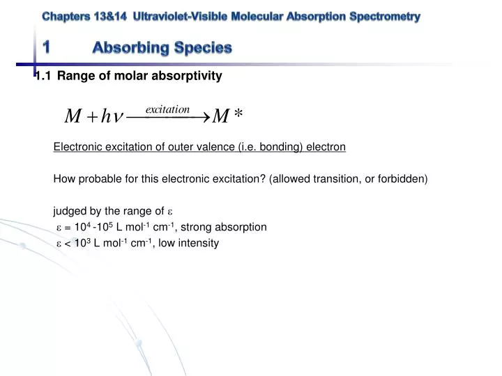
Chapters 13&14 Ultraviolet-Visible Molecular Absorption Spectrometry 1 Absorbing Species. 1.1 Range of molar absorptivity Electronic excitation of outer valence (i.e. bonding) electron How probable for this electronic excitation? (allowed transition, or forbidden)

E N D
Chapters 13&14 Ultraviolet-Visible Molecular Absorption Spectrometry1 Absorbing Species 1.1 Range of molar absorptivity Electronic excitation of outer valence (i.e. bonding) electron How probable for this electronic excitation? (allowed transition, or forbidden) judged by the range of = 104 -105 L mol-1 cm-1, strong absorption < 103 L mol-1 cm-1, low intensity
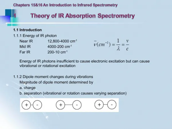
1.2 Which electron get excited? 1.2.1 Organic molecules , (bonding) and n (non-bonding) orbitals *, * (anti-bonding) orbitals * E large ( < 150 nm, out of range) = 10 -10,000 Lmol-1cm-1 n * E smaller ( = 150 - 250 nm) = 200-2000 Lmol-1cm-1 * n * E smallest ( = 200 - 700 nm) = 10-10,000 Lmol-1cm-1 Ideal for UV-Vis spectrometry of organic chromophore
1.2.2 Inorganic molecules Most transition metal ions are colored (absorption in Vis) due to d d electronic transition Fig. 14-4 (p.371) Fig. 14-3 (p.370)
1.2.3 Charge-transfer absorption A: electron donor, metal ions D: electron acceptor, ligand > 10,000 Fig. 14-5 (p.371)
2 Beer’s Law 2.1 Approximation of T and A A = -log T = log (P0/P) = ··b·c : molar absorptivity at one particular wavelength (L·mol-1cm-1) b: path length of absorption (cm) c: molar concentration (mol·L-1) Fig. 6-25 (p.158) Light loss due to reflection (17.3%), scattering, … Fig. 13-1 (p.337)
2.2 Application of Beer’s law to mixtures Absorbance is additive Atotal = A1 + A2 + … = 1bc1 + 2bc2 For a 2-component mixture, we measure the absorption at two different wavelength, respectively A1 = 1,1·b·c1 + 2,1·b·c2 A2 = 1,2·b·c1 + 2,2·b·c2
2.3 Limitations of Beer’s law 2.3.1 Real deviations At low concentration A = -log T = log (P0/P) = ··b·c At c > 0.01 M solute-solute interaction, hydrogen-bond, … can alter the electronic absorption at a given wavelength dilute the solution
2.3.2 Chemical effects analyte associates, dissociates or reacts with a solvent to give molecule with different Example: acid-base equilibrium of an indicator 430 570 HIn 6.30 x10² 7.12x10³ (measured in HCl solution) In- 2.06 x 10⁴ 9.61 x10²(measured in NaOH solution) What’s the absorbance of unbuffered solution at c = 2 x 10⁻⁵M?
Fig. 13-3 (p.340) =[HIn] + [In-]
2.3.3 Instrumental deviations due to polychromatic radiation Beer’s law applies for monochromatic absorption only. If a band of radiation consisting of two wavelength ’, and ” Assuming Beer’s law applies to each wavelength Fig. 7-11 (p.176)
′ ″ ′ ″ ′ ″ 2.3.3 Instrumental deviations due to polychromatic radiation Non-linear calibration curve Fig. 13-4 (p.341)
How to avoid : Select a wavelength band near its maximum absorption where the absorptivity changes little with wavelength Fig. 13-5 (p.341)
2.3.4 Other physical effects stray light – the scattering, reflection radiation from the instrument, outside the nominal wavelength band chosen for measurement mismatched cell for the sample and the blank
3 Noise of Spectrophotometric analyses 3.1 Standard deviation of c
3.2 Sources of instrumental noise Case I Limited readout resolution (31/2-digit displays 0.1% uncertainty from 0%T -100% T) Thermal noise in thermal detector, etc (particularly for IR and neat IR spectrophotometer) Case II Shot noise in photon detector (random emission of photon from the light source or random emission of electrons from the cathode in a detector) Case III Flicker noise, Fail to position sample and blank cells reproducibly in replicate measurements (as a result, different sections of cell window are exposed to radiation, and reflection and scattering losses change)
3.2 Sources of instrumental noise Fig. 13-3 (p.344)
4 Instrumentation 4.1 Designs a. Single beam b. Double-beam-in-space c. Double-beam-in-time Advantage of double beam configuration • Compensate for fluctuation in the radiant output, drift in transducer, etc. • Continuous recording of spectra Fig. 13-13 (p.352)
d. Effects of monchromator exit slit width on spectra Narrow exit slit width improves the spectrum resolution but it also significantly reduce the radiant power Trade-off between resolution and S/N ratio
e. Multichannel spectrometer No monochromator, but disperses transmitted light and measures “all wavelength at once” No Scanning-simple and fast More expensive Limited resolution Fig. 13-15 (p.353)
5 Applications 5.1 Quanlitative spectra Solvent effects on the UV-Vis spectra Polar solvents “blur” vibrational features Polar solvents shift absorption maxima n * blue shift * red shift • - UV-Vis not reliable for qualitative but excellent for quantitative analysis
5.2 Quantitative analysis - Determining the relationship between A and c External Standards Standard-Addition
5.3 Spectrophotometric kinetics Fig. 14-14 (p.382)
Stopped-flow mixing Fig. 14-16 (p.384)