Download

1 / 93
930 likes | 1.15k Vues
Over-complete Representations for Signals/Images. IT 530, Lecture Notes. Introduction: Complete and over-complete bases. Signals are often represented as a linear combination of basis functions (e.g. Fourier or wavelet representation).

E N D
Over-complete Representations for Signals/Images IT 530, Lecture Notes
Introduction: Complete and over-complete bases • Signals are often represented as a linear combination of basis functions (e.g. Fourier or wavelet representation). • The basis functions always have the same dimensionality as the (discrete) signals they represent. • The number of basis vectors is traditionally the same as the dimensionality of the signals they represent. • These bases may be orthonormal (Fourier, wavelet, PCA) or may not be orthonormal (non-orthonormalized ICA).
Introduction: Complete and over-complete bases • A more general representation for signals uses so called “over-complete bases”, where the number of basis functions is MORE than the dimensionality of the signals. • Complete and over-complete bases:
Introduction: Construction of over-complete bases • Over-complete bases can be created by union of multiple sets of complete bases. • Example 1: A signal with n values can be represented using a union of n x n Fourier and n x nHaar wavelet bases, yielding a n x 2n basis matrix. • Example 2: A signal with n values can be represented by adding sinusoids of more frequencies to an existing Fourier basis matrix with n vectors.
Introduction: uniqueness? • With complete bases, the representation of the signal is always unique. • Example: Signals are uniquely defined by their wavelet or Fourier transforms, the eigen-coefficients of any signal (given PCA basis) are uniquely defined. • This uniqueness is LOST with over-complete basis.
Introduction: compactness! • Advantage: over-complete bases afford much greater compactness in signal representation. • Example: Consider two types of audio-signals – whistles and claps. Signals of either type can be represented in a complete Fourier or wavelet basis (power-law of compressibility will apply). • BUT: imagine two complete bases respectively learned for whistles and claps – B1 and B2.
Introduction: compactness! • Suppose B1 and B2 are such that a whistle (resp. clap) signal will likely have a compact representation in the whistle (resp. clap) basis and not in the other one. • A whistle+clap signal will NOT have a compact representation in either basis - B1 or B2 ! • But the whistle+clap signal WILL have a compact representation in the overcomplete basis B = [B1 B2].
More problems • Since a signal can have many representations in an over-complete basis, which one do we pick? • Pick the sparsest one, i.e. the one with least number of non-zero elements which either perfectly reconstructs the signal, or reconstructs the signal up to some error. • Finding the sparsest representation for a signal in an over-complete basis is an NP-hard problem (i.e. the best known algorithm for this task has exponential time complexity )
More problems • In other words, the following problem is NP-hard:
Solving (?) those problems • The NP-hard problem has several methods for approximation – basis pursuit (BP), matching pursuit (MP), orthogonal matching pursuit (OMP) and many others. • None of them will give you the sparsest solution – but they will (under different conditions) yield a solution that is sparse enough.
Bayesian approach • Consider • Assume a suitable prior P(s) on s. • Assume:
Bayesian approach • For zero noise and a Gaussian prior on s, the solution for s is obtained by solving: • For zero noise and a Laplacian prior on s, the solution for s is obtained by solving: Pseudo-inverse Basis Pursuit Approximation
Linear programming: canonical form Linear objective (energy) function Linear equality and inequality constraints
Linear programming for Basis Pursuit Vector of the same size as s, with the negative elements set to 0, and positive elements same as in s. Vector of the same size as s, with the non-negative elements set to 0, and negative elements multiplied by -1 Linear programming problems can be solved in polynomial time! There are various algorithms like simplex (worst-case exponential), interior-point method and ellipsoidal algorithm (both polynomial)
L1 norm and L0 norm • There is a special relationship between the following two problems (which we will study in compressive sensing later on): The L1 norm is a “softer” version of the L0 norm. Other Lp-norms where 0 < p < 1 are possible and impose a stronger form of sparsity, but they lead to non-convex problems. Hence L1 is preferred.
Matching Pursuit • One of the simplest approximation algorithms to obtain the coefficients s of a signal y in an over-complete basis A. • Developed by Mallat and Zhang in 1993 (ref: S. G. Mallat and Z. Zhang, Matching Pursuits with Time-Frequency Dictionaries, IEEE Transactions on Signal Processing, December 1993) • Based on successively choosing that vector in A which has maximal inner product with a so-called residual vector (initialized to y in the beginning).
Pseudo-code “j” or “l” is an index for dictionary columns
Properties of matching pursuit • The reconstruction error, i.e. is always guaranteed to decrease. The decrease is at an exponential rate. • At any iteration, the following relationship holds true:
Orthogonal Matching Pursuit (OMP) • More sophisticated algorithm as compared to matching pursuit (MP). • The signal is approximated by successive projection onto those dictionary columns (i.e. columns of A) that are associated with a current “support set”. • The support set is also successively updated.
Pseudo-code Support set Several coefficients are re-computed in each iteration Sub-matrix containing only those columns which lie in the support set
OMP versus MP • Unlike MP, OMP never re-selects any element. • Unlike MP, in OMP, the residual at an iteration is always orthogonal to all currently selected elements. • OMP is costlier per iteration (due to pseudo-inverse ) but generally more accurate than MP. • Unlike MP, OMP converges in K iterations for a dictionary with K elements. • OMP always gives the optimal approximation w.r.t. the selected subset of the dictionary (note: this does not mean that the selected subset itself was optimal).
OMP and MP for noisy signals • It is trivial to extend OMP and MP for noisy signals. • The stopping criterion is a small residual magnitude e (not zero).
BP under noise A quadratic programming problem that is structurally similar to a linear program
Learning the bases • So far we assumed that the basis (i.e. A) was fixed, and optimized for the sparse representation. • Now, we need to learn A as well! • We’ve learned about PCA, ICA. But they don’t always give the best representation!
PCA ICA Over-complete ICA
Learning the bases: analogy with K-means • In K-means, we start with a bunch of K cluster centers and assign each point in the dataset to the nearest cluster center. • The cluster centers are re-computed by taking the mean of all points assigned to a cluster. • The assignment and cluster-center computation problems are iterated until a convergence criterion is met.
Learning the bases: analogy with K-means • K-means is a special sparse coding problem where each point is represented by strictly one of K dictionary elements. • Our dictionary (or bases) learning problem is more complex: we are trying to express each point as a linear combination of a subset of dictionary elements (or a sparse linear combination of dictionary elements).
Learning the Bases! • Find model (i.e. over-complete basis) A for which the likelihood of the data is maximized. • Above integral is not available in closed form for most priors on s (e.g. Laplacian - intractable). • Approximation (Method 1): Assume that the volume of the pdf is concentrated around the mode (w.r.t. s). Ref: Olshausen and Field, “Natural image statistics and efficient coding”
Two-step iterative procedure • Fix the basis A and obtain the sparse coefficients for each signal using MP, OMP or BP (some papers – like the one by Olshausen and Field - use gradient descent for this step!). • Now fix the coefficients, and update the basis vectors (using various techniques, one of which was described on the previous slide). • Normalize each basis vector to unit norm. • Repeat the previous two steps until some error criterion is met.
Toy Experiment 1 Result of basis learning (dictionary with 144 elements) with sparsity constraints on the codes. Training performed on 12 x 12 patches extracted from natural images. Ref: Olshausen and Field, “Natural image statistics and efficient coding”
Toy Experiment 2 • Data-points generated as a (Laplacian/super-Laplacian) random linear combination of some arbitrarily chosen basis vectors. • In the no-noise situation, the aim is to extract the basis vectors and the coefficients of the linear combination. • The fitting results are shown on the next slide. The true and estimated directions agree quite well. Ref: Lewicki and Sejnowski, “Learning overcomplete representations”
Learning the Bases: Method of Optimal Directions (MOD) - Method 2 • Given a fixed dictionary A, assume sparse codes for every signal are computed using OMP, MP etc. • The overall error is now given as • We want to find dictionary A that minimizes this error. Ref: Engan et al, “Method of optimal directions for frame design”
Learning the Bases: Method of Optimal Directions (MOD) - Method 2 • Take the derivative of E(A) w.r.t. A and set it to 0. This gives us the following update: • Following the update of A, each column in A is independently rescaled to unit norm. • The updates of A and S alternate with each other till some convergence criterion is reached. • This method is more efficient than the one by Olshausen and Field.
Learning the Bases: Method 3- Union of Orthonormal Bases • Like before, we represent a signal in the following way: • A is an over-complete dictionary, but let us assume that it is a union of ortho-normal bases, in the form
Learning the Bases: Method 3- Union of Ortho-normal Bases • The coefficient matrix S can now be written as follows (M subsets, each corresponding to a single orthonormal basis): • Assuming we have fixed bases stored in A, the coefficients in S can be estimated using block coordinate descent, described on the following slide.
Learning the Bases: Method 3- Union of Ortho-normal Bases There is a quick way of performing this optimization given an ortho-normal basis – SOFT THRESHOLDING (could be replaced by hard thresholding if you had a stronger sparseness prior than an L1 norm
Learning the Bases: Method 3- Union of Ortho-normal Bases • Given the coefficients, we now want to update the dictionary which is done as follows: Why are we doing this? It is related to the so-called orthogonal Procrustes problem - a well-known application of SVD. We will see this on the next slide. The specific problem we are solving is given below. Note that it cannot be solved using a pseudo-inverse as that will not impose orthonormality constraint, if there is noise in the data or if the coefficients are perturbed or thresholded.
Learning the Bases: Method 3- Union of Ortho-normal Bases • Keeping all bases in A fixed, update the coefficients in S using a known sparse coding technique. • Keeping the coefficients in S fixed, update the bases in A using the aforementioned SVD-based method. • Repeat the above two steps until a convergence criterion is reached.
Learning the Bases: Method 4 – K-SVD • Recall: we want to learn a dictionary and sparse codes on that dictionary given some data-points: • Starting with a fixed dictionary, sparse coding follows as usual – OMP, BP, MP etc. The criterion could be based on reconstruction error or L0-norm of the sparse codes. • The dictionary is updated one column at a time.
Row ‘k’ (NOT column) of matrix S Does NOT depend on the k-th dictionary column How to find ak, given the above expression? We have decomposed the original error matrix, i.e. Y-AS, into a sum of rank-1 matrices, out of which only the last term depends on ak. So we are trying to find a rank-1 approximation for Ek, and this can be done by computing the SVD of Ek, and using the singular vectors corresponding to the largest singular value.
Problem! The dictionary codes may no more be sparse! SVD does not have any in-built sparsity constraint in it! So, we proceed as follows: Considers only those columns of Y (i.e. only those data-points) that actually USE the k-th dictionary atom, effectively yielding a smaller matrix, of size p by |wk| Consider the error matrix defined as follows: This update affects the sparse codes of only those data-points that used the k-th dictionary element
KSVD and K-means • Limit the sparsity factor T0 = 1. • Enforce all the sparse codes to be either 0 or 1. • Then you get the K-means algorithm!
Implementation issues • KSVD is a popular and effective method. But some implementation issues haunt K-SVD (life is never easy ). • KSVD is susceptible to local minima and over-fitting if K is too large (just like you can get meaningless clusters if your number of cluster is too small, or get meaningless densities if the number of histogram bins is too many). • KSVD convergence is not fully guaranteed. The dictionary updates given fixed sparse codes ensure the error decreases. However the sparse codes given fixed dictionary may not decrease the error – it is affected by the behaviour of the sparse coding approximation algorithms. • You can speed up the algorithm by removing extremely “unpopular” dictionary elements, or removing duplicate (or near-duplicate) columns of the dictionary.
(Many) Applications of KSVD • Image denoising • Image inpainting • Image deblurring • Blind compressive sensing • Classification • Compression • And you can work on many more
Application: Image Compression (Training Phase) • Training set for dictionary learning: a set of 11000 patches of size 8 x 8 – taken from a face image database. Dictionary size K = 441 atoms (elements). • OMP used in the sparse coding step during training – stopping criterion is a fixed number of coefficients T0 = 10. • Over-complete Haar and DCT dictionaries – of size 64 x 441 – and ortho-normal DCT basis of size 64 x 64 (JPEG), also used for comparison.
Application: Image Compression (Testing Phase) • A lossy image compression algorithm is evaluated using an ROC curve – the X axis contains the average number of bits to store the signal. The Y-axis is the associated error or PSNR. Normally, the acceptable error is fixed and the number of bits is calculated. • The test image is divided into non-overlapping patches of size 8 x 8. • Each patch is projected onto the trained dictionary and its sparse code is obtained using OMP given a fixed error e.