Download
1 / 34
400 likes | 1.55k Vues
Fundamentals of Audio Signals Two signals of different amplitudes A greater amplitude represents a louder sound. Fundamentals of Audio Signals Two signals of different frequencies A greater frequency represents a higher pitched sound. Fundamentals of Audio Signals

E N D
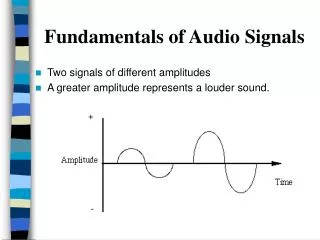
Fundamentals of Audio Signals • Two signals of different amplitudes • A greater amplitude represents a louder sound.
Fundamentals of Audio Signals • Two signals of different frequencies • A greater frequency represents a higher pitched sound.
Fundamentals of Audio Signals • Any sound, no matter how complex, can be represented by a waveform. • For complex sounds, the waveform is built up by the superposition of less complex waveforms • The component waveforms can be discovered by applying the Fourier Transform • Converts the signal to the frequency domain • Inverse Fourier Transform converts back to the time domain
Sampling • Sounds can be thought of as functions of a single variable (t) which must be sampled and quantized • The sampling rate is given in terms of samples per second, or, kHz • During the sampling process, an analog signal is sampled at discrete intervals • At each interval, the signal is momentarily “held” and represents a measurable voltage rate
Quantization • Audio is usually quantized at between 8 and 20 bits • Voice data is usually quantized at 8 bits • Professional audio uses 16 bits • Digital signal processors will often use a 24 or 32 bit structure internally
Quantization • The accuracy of the digital encoding can be approximated by considering the word length per sample • This accuracy is known as the signal-to-error ratio (S/E) and is given by: • S/E = 6n + 1.8 dB • n is the number of bits per sample
Quantization • When a coarse quantization is used, it may be useful to add a high-frequency signal (analog white noise) to the signal before it is quantized • This will make the coarse quantization less perceptible when the signal is played back • This technique is known as dithering • During the sampling process, an analog signal is sampled at discrete intervals • At each interval, the signal is momentarily “held” and represents a measurable voltage rate
Channels • We may also have audio data coming from more than one channels • Data from a multichannel source is usually interleaved • Sampling rates are always measured per channel • Stereo data recorded at 8000 samples/second will actually generate 16,000 samples every second
Digital Audio Data • A complete description of digital audio data includes (at least): • sampling rate; • number of bits per sample; • number of channels (1 for mono, 2 for stereo, etc.)
Analog to Digital Conversion • Nyquist’s theorem states that if an arbitrary signal has been run through a low-pass filter of bandwidth H, the filtered signal can be completely reconstructed by making only 2H (exact) samples per second. • So, a low-pass filter is placed before the sampling circuitry of the analog-to-digital (A/D) converter.
Analog to Digital Conversion • If frequencies greater than the Nyquist limit enter the digitization process, an unwanted condition called aliasing occurs • The low-pass filter used will require the use of a gradual high-frequency roll-off, thus a sampling rate somewhat higher than twice the Nyquist limit is often used • A/D conversion may make use of a successive approximation register (SAR)
Analog to Digital Conversion • The low-pass filter can cause side effects. • One way that these side effects can be overcome is through the use of oversampling - a signal-processing function that raises the sample rate of a digitally encoded signal. • Consumer and professional 16-bit D/A converters often use up to 8- and 12-times oversampling, raising the sampling rate of a CD (for example) from 44.1 kHz to 352.8 kHz or 529.2 kHz. • By altering the signal’s noise characteristics, it is possible to shift much of the overall bandwidth noise out of the range of human hearing.
Pulse Code Modulation • The method that has been discussed for storing audio is known as pulse code modulation (PCM).
Pulse Code Modulation • PCM is common in long-distance telephone lines. • The analog signal (voice) is sampled at 8000 samples/second with 7 or 8 bits per sample • A T1 carrier handles 24 voice channels multiplexed together • The bandwidth of this type of carrier can be calculated as follows: • 8 bits x 8000 samples/second x 24 channels = 1.544 Mbps • Note that one out of 8 bits is for control, not data.
Pulse Code Modulation • D/A conversion process • parallelize the serial bit stream • generate an analog voltage analogous to the voltage level at the original time of sampling • An output sample and hold circuit is used to minimize spurious signal glitches • a final low-pass filter is inserted into the path • Smooths out the non-linear steps introduced by digital sampling
Pulse Code Modulation • Other PCM topics: • mu-law and A-law companding • DPCM • DM • ADPCM
Digital Signal Processing • Processing of a digital signal to achieve special effects may generally be described in terms of some simple functions: • Addition • Multiplication • Delay • Resampling
Digital Signal Processing • Addition of two signals is accomplished by adding the sample values of the signals at each sampling point: h(t)=f(t)+g(t) • We can add as many signals as desired together • Multiplication of a given signal is represented as: g(t)=m*f(t), where m is the multiplication factor. • Multiplication is used to increase or decrease the gain (loudness) of a signal. If m>1, g is louder than f. If m<1, g is less loud than f • Note that when adding signals together or multiplying by a number greater than one, care must be taken when the signal reaches the upper limit of the sample size
Digital Signal Processing • Delay is an important effect described as follows: g(t)=f(t+d), where d is a delay time • Use delay and addition to model echo: • f(t) = HELLO • g(t) = f(t + d1) , where 0 <d1 • g(t) = HELLO • h(t) = f(t + d2) , where 0 <d1 < d2 • h(t) = HELLO • F(t) = f(t) + g(t) + h(t) • = HELLO HELLO HELLO
Digital Signal Processing • Now consider a more realistic echo effect. We need to make each succeeding echo softer. We can do this with multiplication. • g’(t) = m*g(t)h’(t) = n*h(t), 0<n<m<1 • F’(t) = f(t) + g’(t) + h’(t) = HELLO HELLOHELLO
Digital Signal Processing • When delays of 35-40 ms and greater are used, the listener perceives them as discrete delays • Reducing the delay to the 15-35 ms range will create delays that are too closely spaced to be perceived as discrete delays • When used with instruments, the brain is fooled into thinking that more instruments are playing than there actually are • combining several short term delay modules that are slightly detuned in time, an effect known as chorusing can be achieved (used by guitarists, e.g.)
Pitch-Related Effects • DSP functions are available that can alter the speed and pitch of an audio program. These can: • Change pitch without changing duration • Change duration without changing pitch • Change both duration and pitch • The process for raising and lowering the pitch of a sample is shown on the next slides
Noise Elimination • The noise elimination process can be seen to consist of three steps: • Visual analysis • De-clicking • De-noising • Use visual analysis to determine the type of noise and to guide the next two steps
Noise Elimination • De-clicking involves the removal of noise generated by analog side effects such as tape hiss, needle ticks, pops, etc. • This is similar to ‘snow’ removal in image processing • (the noise manifests itself as large discontinuities in the sample waveform) • The noise is likely to have affected more sample data in the audio file than in the corresponding image file • A needle skip which affects 1/4 second of the file affects 11000 samples at the audio CD sampling rate • Therefore, reconstruction of the affected area is not the straightforward linear interpolation process used in images • Must examine a large portion of the waveform to reconstruct
Noise Elimination • De-noising involves the removal of background noise such as hum, buzzes, air-conditioner noises, etc • The waveform is analyzed to determine if louder sounds will mask the softer sound • This involves breaking down the audio spectrum into a large number of frequency bands • The signal is compared with a signature which represents the background noise. This is taken from a silent moment in the samplefile. It must be determined which portion of a signal is noise and whether the noise can be deleted without distorting the program
Digital Signal Processing • Other DSP functions include digital mixing and sample rate conversion • Digital mixing is the integration of a number of digital audio signals into a single ouput signal • Sample rate conversion is necessary when a signal sampled at one rate must be played back on or transferred to equipment which uses another rate • An example is the use of digital audio as the sound track for video. The incoming rate of 44.1 kHz must be “pulled-down” to 44.056 kHz
Fading • Fading is another important DSP function • During a fade, the calculated sample amplitudes are either proportionately reduced or proportionately increased in level, according to a defined curve ramp • For example, usually when performing a fade out, the signal will begin at a level that is 100 percent of its current value and will reduce over the defined time to 0 percent • Examples of various fade curves are shown in the following slides
Fading • To find the linearly faded value of a sample at time tx, t0≤tx≤t1, we use the following equation: • s’(tx) = s(tx) * (tx - t0) / (t1 - t0) • We can also combine the fade in of one soundfile with the fade out of another soundfile to produce the effect known as crossfade
Fading • Note that the two curves intersect at 50% attenuation and that the sum of the two values at any point in time is always 100% • Thus, we can add together the two signals to form our crossfaded signal and the amplitude of the waveform will never be greater than the maximum possible amplitude