Statistics Measures of Central Tendency

1. StatisticsMeasures of Central Tendency

2. Why Describe Central Tendency? • Data often cluster around a central value that lies between the two extremes. This single number can describe the value of scores in the entire data set. • There are three measures of central tendency. 1) Mean 2) Median 3) Mode

3. Measures of central tendency are scores that represent the center of the distribution. Three of the most common measures of central tendency are: Mean Median Mode

4. Mean The most commonly used measure of central tendency When people ask about the “average” of a group of scores, they usually are referring to the mean. The mean is the sum of all the scores in the distribution divided by the total scores (the mathematical average).

5. Mean (con’t) Mean of a sample Mean of a population

6. Mean (con’t) Exam Scores n = total number of scores for the sample

7. Mean - Ungrouped Data Mean - Grouped Data For a population: For a population: å fX m = + + + + X X X ... X å X 1 2 3 N N m = = N N For a sample: For a sample: å fX = X + + + + X X X ... X å X n 1 2 3 n = = X n n Formula 7.A Formula 7.B Arithmetic Mean 7.7

8. Mean (con’t) The mean includes the weight of every score.

9. Table 7.2 | Approximation of the Arithmetic Mean from a Frequency Distribution Absolute Class Class Frequency (number Class (net profit in of companies in Midpoint millions of rupees) class) f X fX -1,250 to under 0 6 -625 -3,750 0 to under 1,250 49 625 30,625 1,250 to under 2,500 18 1,875 33,750 2,500 to under 3,750 15 3,125 46,875 3,750 to under 5,000 3 4,375 13,125 5,000 to under 6,250 2 5,625 11,250 6,250 to under 7,500 4 6,875 27,500 7,500 to under 8,750 2 8,125 16,250 8,750 to under 1 9,375 9,375 S S 10,000 f = N = 100 fX = 185,000 Estimated arithmetic mean = Rs.1,850 (based on the ratio 185,000/100) Table 7.2 Arithmetic Mean 7.9

10. Pros and cons of using mean Pros Summarizes data in a way that is easy to understand. Uses all the data Used in many statistical applications Cons Affected by extreme values E.g., average salary at a company 12,000; 12,000; 12,000; 12,000; 12,000; 12,000; 12,000; 12,000; 12,000; 12,000; 20,000; 390,000 Mean = $44,167

11. Merits and demerits of mean • Merits • Mean is well understood by most people • Computation of mean is easy • Demerits • Sensitive to extreme value • For example: • X={1,1,1,1,2,9}, mean(X)=2.5 which does not reflect the actually central tendency of this set of numbers

12. Median The middle score of the distribution when all the scores have been ranked. If there are an even number of scores, the median is the average of the two middle scores.

13. Median • Definition • It divides the numbers into two halves such that the number of items below it is the same as the number of items above it • Suppose we have n numbers x1, x2, ……, xn. • Median is defined as

14. Median (con’t) Number of Words Recalled in Performance Study

15. Median - Ungrouped Data Median - Grouped Data For a population: For a population: - ( N / 2 ) F M = M = + X L w + N 1 f 2 For a sample: For a sample: - ( n / 2 ) F = m X + = + n 1 m L w f 2 L = the median class’s lower limit X = population (or sample) value f = its absolute frequency N = number of observations in population w = its width n = number of observations in sample F = the sum of frequencies up to subscript = position of X in ordered array (but not including) those of the median class Formula 7.C Formula 7.D The Median 7.15

16. Merits and demerits of median • Merits • Another widely used measure of central tendency • It is not influenced by extreme values • Demerits • When the number of items are small, median may not be representative, because it is a positional average

17. Mode The most frequent score in the distribution. A distribution where a single score is most frequent has one mode and is called unimodal. A distribution that consists of only one of each score has n modes. When there are ties for the most frequent score, the distribution is bimodal if two scores tie or multimodal if more than two scores tie.

18. Mode (con’t) Number of Words Recalled in Performance Study The mode is 4.

19. Mode (con’t) This distribution is bimodal. Demonstration

20. Calculations • Key: dependent measure is reaction time • Time it takes to say the color • Determine the mean, median, and mode of the datasets in the handout.

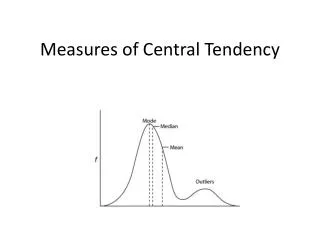
21. Shape of the Distribution Skew refers to the general shape of a distribution when it is graphed. Symmetrical = zero skew Scores clustered on the high or low end of a distribution = skewed distribution

22. The mean, median, and mode are the same.

23. The normal distribution is the “ideal” symmetrical distribution

24. Distributions that are skewed have one side of the distribution where the data frequency tapers off

25. Skewed Distribution Tail points in the positive direction.

26. Skewed Distribution Tail points in negative direction.

27. The mean will either underestimate or overestimate the center of skewed distributions. Mode Mode Median Median Mean Mean

28. Kurtosis Measure of the flatness or peakedness of the distribution

29. Measures of Location • Measures that are allied to the median include the quartiles, deciles and percentiles, because they are also based on their position in a series of observations. • These measures are referred to as measures of location and not the measures of central tendency as they describe the position of one score relative to the others rather than the whole set of data.

30. Measures of Location • Quartile • One fourth (1/4) • First (1/4), Second (1/2), Third (3/4) • Decile • One tenth (1/10) • 10%, 20%, …90% • Percentile • One of hundreds (1/100) • 1%, 2%, ….99%

31. Quartiles • The median divides the data into two equal sets. • The lower quartile is the value of the middle of the first set, where 25% of the values are smaller than Q1 and 75% are larger. This first quartile takes the notation Q1. • The upper quartile is the value of the middle of the second set, where 75% of the values are smaller than Q3 and 25% are larger. This third quartile takes the notation Q3.

32. Quartiles • Example 1 – Upper and lower quartiles • Data • 6, 47, 49, 15, 43, 41, 7, 39, 43, 41, 36 • Ordered data • 6, 7, 15, 36, 39, 41, 41, 43, 43, 47, 49 • Median 41 • Upper quartile 43 • Lower quartile 15

33. Quartile • L0 = Lower limit of the i-th Quartile class • n = Total number of observations in the distribution • h = Class width of the i-th Quartile class • fi = Frequency of the i-th Quartile class • F = Cumulative frequency of the class prior to the i-th quartile class

34. Decile • L0 = Lower limit of the i-th Decile class • n = Total number of observations in the distribution • h = Class width of the i-th Decile class • fi = Frequency of the i-th Decile class • F = Cumulative frequency of the class prior to the i-th Decile class

35. Percentile • L0 = Lower limit of the i-th Percentile class • n = Total number of observations in the distribution • h = Class width of the i-th Percentile class • fi = Frequency of the i-th Percentile class • F = Cumulative frequency of the class prior to the i-th Percentile class

36. Example-1: Percentile of Ungroup data • Consider the observations 11, 14, 17, 23, 27, 32, 40, 49, 54, 59, 71 and 80. To determine the 29th percentile? • we note that which is not an integer. Thus the next higher integer 4 here will determine the 29th percentile value. On inspection P29 = 23

37. Example-2: Find 3rd Quartiles, 1st Decile and 29th Percentile

38. Example-3: Find 30th percentile

39. Determine Percentile Class • First determine the percentile class. • If, N =5736, and we have to find 30th percentile, then percentile class will be the class which has cumulative frequency below:

40. 30th Percentile class 1728.9

41. Percentiles and Location Top of 1st Q-tile Top of 2nd Q-tile (med) Top of 3rd Q-tile 25th percentile 50th percentile 75th percentile If you’re at the 75th percentile, or the 3rd quartile, of test scores this means 75% of other test takers scored below you. Which is a better score, 1st percentile or 99th percentile?

42. A box plot is a graphical display, based on quartiles, that helps to picture a set of data. Five pieces of data are needed to construct a box plot: • the Minimum Value, • the First Quartile, • the Median, • the Third Quartile, and • the Maximum Value. Box Plots

43. Based on a sample of 20 deliveries, Buddy’s Pizza determined the following information. The minimum delivery time was 13 minutes and the maximum 30 minutes. The first quartile was 15 minutes, the median 18 minutes, and the third quartile 22 minutes. Develop a box plot for the delivery times. Example 4

44. Example 4 continued