Chi Square Fitting – C ode for Fitting w (z ) with Data
Chi Square Fitting – C ode for Fitting w (z ) with Data . Pao -Yu Wang. Outline. Introduction Basic methods and derivations Chi-square fitting: some techniques Brief introduction of the code ROOT Results. Introduction. The universe is expanding at late times

Chi Square Fitting – C ode for Fitting w (z ) with Data
E N D
Presentation Transcript
Chi Square Fitting –Code for Fittingw(z) with Data Pao-Yu Wang
Outline • Introduction • Basic methods and derivations • Chi-square fitting: some techniques • Brief introduction of the code • ROOT • Results
Introduction • The universe is expanding at late times • Needs extra energy density source with negative pressure • Many different models had been proposed: • Cosmological constant • Quintessence • Phantom • … • Observations constrain the behaviors of dark energy!
The basics and methods • Parametrization: (0 < z < 1) • We want to constrain this by data! • SN 1a, CMB(WMAP), BAO(SDSS,2dFGRS) • Models can also give predictions of w(z) • Ex: for ΛCDM, • Then we can compare data with models
The basics and methods: how to constrain? • Let’s return to math first: • Distance module (SN 1a): Now
H(z) can further be expressed as (using the parametrization): • Plug in this back to dL, we then will have μ can be derived from 4 parameters in theory μ can be observed directly Then we can compare data with models!
χ-Square fitting • For SN 1a, μ is measureable • CMB: shift parameter R is measureable! • BAO: Observation can give DV(0.35)/DV(0.2)
Data set we use… • Old dataset: • New dataset: From: SEVEN-YEAR WILKINSON MICROWAVE ANISOTROPY PROBE (WMAP1) OBSERVATIONS: COSMOLOGICAL INTERPRETATION, ArXiv: 1001.4538v2 From: Baryon Acoustic Oscillations in the Sloan Digital Sky Survey Data Release 7 Galaxy Sample, ArXiv: 0907.1660v3
PDG -- Statistics • From χ-square fitting we will get a best fit point
Brief Introduction of the Code • By Chien-Wen Chen • Using ROOT library • Calculate theoretical value Calculate χ-square • Use ROOT to find best fit and draw diagrams, contours
ROOT • “ROOT is an object oriented framework for large scale data analysis” • Can be used to draw plots, histograms, find best fit, etc. • An simple example:
Start ROOT at terminal: Other example: 3D In Chien-Wen’s code we use makefile directly.
Results • Best fit and error: • Using WMAP 5 years BAO(2007) • And now we have New data… Old best fit w0= -0.912977 wa= -0.231426 M= 0.268077 errw0+= 0.13023 errw0-= -0.146007 errwa+= 0.756889 errwa-= -0.783501 ……
All with 68.3%, 95.4% confidence level Old plot New plot • 1
Next thing to do… • w-w’ plane • Different models can have different region in this This is from models! Now we convert our w0-wa plane into w-w’ plane