Priority Queues (Heaps) Analysis and Implementations
Learn about modeling, simple implementations, binary heaps, d-heaps, leftist heaps, skew heaps, binomial queues, and more in priority queues (heaps) along with applications and standard library usage. Understand heap structure, heap-order property, and basic and other operations. Explore array implementation and the priority queue interface.

Priority Queues (Heaps) Analysis and Implementations
E N D
Presentation Transcript
Data Structure and Algorithm Analysis06: Priority Queue (Heaps) http://net.pku.edu.cn/~course/cs202/2014 Hongfei Yan School of EECS, Peking University 4/23/2014
Contents 01 Programming: A General Overview (20-65) 02 Algorithm Analysis (70-89) 03 Lists, Stacks, and Queues (96-135) 04 Trees (140-200) 05 Hashing (212-255) 06 Priority Queues (Heaps) (264-302) 07 Sorting (310-360) 08 The Disjoint Sets Class (370-393) 09 Graph Algorithms (398-456) 10 Algorithm Design Techniques (468-537)
Motivation • Jobs sent to a printer are generally placed on a queue, • one job might be particularly important • Conversely, if there are several 1-page jobs and one 100-page job, it might be reasonable to make the long job go last, even if it is not the last job submitted. • In a multiuser environment, the operating system scheduler must decide which of several processes to run. • Generally, it is important that short jobs finish as fast as possible • some jobs that are not short are still very important and should also have precedence. • require a special kind of queue, known as a priority queue.
02 Priority Queues (Heaps) 6.1 Model 6.2 Simple Implementations 6.3 Binary Heap 6.4 Applications of Priority Queues 6.5 d-Heaps 6.6 Leftist Heaps 6.7 Skew Heaps 6.8 Binomial Queues 6.9 Priority Queues in the Standard Library
Basic model of a priority queue • allows at least the following two operations: • insert, which does the obvious thing; • And deleteMin, which finds, returns, and removes the minimum element in the priority queue.
02 Priority Queues (Heaps) 6.1 Model 6.2 Simple Implementations 6.3 Binary Heap 6.4 Applications of Priority Queues 6.5 d-Heaps 6.6 Leftist Heaps 6.7 Skew Heaps 6.8 Binomial Queues 6.9 Priority Queues in the Standard Library
several obvious ways to implement a priority queue • use a simple linked list, • performing insertions at the front in O(1) and traversing the list, which requires O(N) time, to delete the minimum. • Alternatively, the list be kept always sorted; this makes insertions expensive (O(N)) and deleteMins cheap (O(1)). • The former is probably the better idea of the two, based on the fact that there are never more deleteMins than insertions. • Another way of implementing priority queues would be to use a binary search tree. • This gives an O(logN) average running time for both operations. • Repeatedly removing a node that is in the left subtree would seem to hurt the balance of the tree by making the right subtree heavy • Using a search tree could be overkill because it supports a host of operations that are not required.
02 Priority Queues (Heaps) 6.1 Model 6.2 Simple Implementations 6.3 Binary Heap 6.4 Applications of Priority Queues 6.5 d-Heaps 6.6 Leftist Heaps 6.7 Skew Heaps 6.8 Binomial Queues 6.9 Priority Queues in the Standard Library
Binary Heap merely as Heap • The priority queue is known as a binary heap. • Heaps have two properties, namely, a structure property and a heaporder property. • As with AVL trees, an operation on a heap can destroy one of the properties, • so a heap operation must not terminate until all heap properties are in order.
6.3 Binary Heap 6.3.1 Structure Property 6.3.2 Heap-Order Property 6.3.3 Basic Heap Operations 6.3.4 Other Heap Operations
Complete Binary Tree • A heap is a binary tree that is completely filled, with the possible exception of the bottom level, which is filled from left to right. Such a tree is known as a complete binary tree. • a complete binary tree of height h has between 2h and 2h+1 − 1 nodes. • This implies that the height of a complete binary tree is , which is clearly O(logN).
Array implementation of complete binary tree (1/2) An important observation is that because a complete binary tree is so regular, it can be represented in an array and no links are necessary.
Array implementation of complete binary tree (2/2) • For any element in array position i, • the left child is in position 2i, • the right child is in the cell after the left child (2i + 1), • and the parent is in position i/2. • Thus, not only are links not required, but the operations required to traverse the tree are extremely simple and likely to be very fast on most computers. • The only problem with this implementation is that an estimate of the maximum heap size is required in advance, • but typically this is not a problem (and we can resize if needed). • A heap data structure will, then, consist of an array (of Comparable objects) and an integer representing the current heap size. • we shall draw the heaps as trees, with the implication that an actual implementation will use simple arrays.
6.3.2 Heap-Order Property • The property that allows operations to be performed quickly is the heap-order property. • Since we want to be able to find the minimum quickly, it makes sense that the smallest element should be at the root. • If we consider that any subtree should also be a heap, then any node should be smaller than all of its descendants.
6.3 Binary Heap 6.3.1 Structure Property 6.3.2 Heap-Order Property 6.3.3 Basic Heap Operations 6.3.4 Other Heap Operations
Insertion operation To insert an element X into the heap, we create a hole in the next available location This general strategy is known as a percolate up; the new element is percolated up the heap until the correct location is found.
deleteMin • deleteMins are handled in a similar manner as insertions. • Finding the minimum is easy; the hard part is removing it. • When the minimum is removed, a hole is created at the root. • Since the heap now becomes one smaller, it follows that the last element X in the heap must move somewhere in the heap. • If X can be placed in the hole, then we are done. This is unlikely, so we slide the smaller of the hole’s children into the hole, thus pushing the hole down one level. • We repeat this step until X can be placed in the hole. Thus, our action is to place X in its correct spot along a path from the root containing minimum children.
Method to perform deleteMin in a binary heap (2/2) A frequent implementation error in heaps occurs when there are an even number of elements in the heap, and the one node that has only one child is encountered. You must make sure not to assume that there are always two children, so this usually involves an extra test.
6.3.4 Other Heap Operations • a heap has very little ordering information • no way to find any particular element without a linear scan through the entire heap. • if it is important to know where elements are, • some other data structure, such as a hash table, must be used in addition to the heap. • If we assume that the position of every element is known by some other method, • then several other operations become cheap. • The first three operations below all run in logarithmic worst-case time.
decreaseKey • The decreaseKey(p,∆) operation lowers the value of the item at position p by a positive amount ∆. • Since this might violate the heap order, it must be fixed by a percolate up. • This operation could be useful to system administrators: They can make their programs run with highest priority
increaseKey The increaseKey(p, ∆) operation increases the value of the item at position p by a positive amount ∆. This is done with a percolate down. Many schedulers automatically drop the priority of a process that is consuming excessive CPU time.
remove • The remove(p) operation removes the node at position p from the heap. • This is done by first performing decreaseKey(p,∞) • and then performing deleteMin(). • When a process is terminated by a user (instead of finishing normally), it must be removed from the priority queue.
buildHeap (1/2) • constructed from an initial collection of items. This constructor takes as input N items and places them into a heap. • Obviously, this can be done with N successive inserts. • Since each insert will take O(1) average and O(logN) worst-case time, • the total running time of this algorithm would be O(N) average but O(N logN) worst-case. • we already know that the instruction can be performed in linear average time
buildHeap (2/2) • The general algorithm is to place the N items into the tree in any order, maintaining the structure property. • Then, if percolateDown(i) percolates down from node i, the buildHeap routine in Figure 6.14 can be used by the constructor to create a heap-ordered tree. • To bound the running time of buildHeap, we must bound the number of dashed lines. • This can be done by computing the sum of the heights of all the nodes in the heap, • which is the maximum number of dashed lines. What we would like to show is that this sum is O(N).
Theorem 6.1 For the perfect binary tree of height h containing 2h+1−1 nodes, the sum of the heights of the nodes is 2h+1 − 1 − (h + 1). Proof It is easy to see that this tree consists of 1 node at height h, 2 nodes at height h − 1, 22 nodes at height h − 2, and in general 2inodes at height h − i. The sum of the heights of all the nodes is then
buildHeap is linear • A complete tree is not a perfect binary tree, but the result we have obtained is an upper bound on the sum of the heights of the nodes in a complete tree. • Since a complete tree has between 2h and 2h+1 nodes, this theorem implies that this sum is O(N), where N is the number of nodes. • Although the result we have obtained is sufficient to show that buildHeap is linear, the bound on the sum of the heights is not as strong as possible. • For a complete tree with N = 2h nodes, the bound we have obtained is roughly 2N. • The sum of the heights can be shown by induction to be N − b(N), where b(N) is the number of 1s in the binary representation of N.
02 Priority Queues (Heaps) 6.1 Model 6.2 Simple Implementations 6.3 Binary Heap 6.4 Applications of Priority Queues 6.5 d-Heaps 6.6 Leftist Heaps 6.7 Skew Heaps 6.8 Binomial Queues 6.9 Priority Queues in the Standard Library
6.4.1 The Selection Problem • The input is a list of N elements, which can be totally ordered, and an integer k. The selection problem is to find the kth largest element. • algorithm 1A, is to read the elements into an array and sort them, returning the appropriate element. Assuming a simple sorting algorithm, the running time is O(N2). • The 1B, is to read k elements into an array and sort them. • process the remaining elements one by one. As an element arrives, it is compared with the kth element in the array. • If it is larger, then the kth element is removed, and the new element is placed in the correct place among the remaining k−1 elements. • When the algorithm ends, the element in the kth position is the answer. The running time is O(N·k) • If , then both algorithms are O(N2). • This also happens to be the most interesting case, since this value of k is known as the median.
Median • The middle number (in a sorted list of numbers). • To find the Median, place the numbers you are given in value order and find the middle number. • Example: find the Median of {13, 23, 11, 16, 15, 10, 26}. • Put them in order: {10, 11, 13, 15, 16, 23, 26} • The middle number is 15, so the median is 15. • (If there are two middle numbers, you average them.)
Algorithm 6A • assume that we are interested in finding the kth smallest element. • read the N elements into an array. • apply the buildHeap algorithm to this array. • perform k deleteMin operations. • obtain a total running time of O(N + k logN). • If k = O(N/logN), then the running time is dominated by the buildHeap operation and is O(N). • For larger values of k, the running time is O(k logN). If , then the running time is (N logN). • Notice that if we run this program for k = N and record the values as they leave the heap, we will have essentially sorted the input file in O(N logN) time.
Algorithm 6B (1/2) • maintain a set S of the k largest elements. • After the first k elements are read, when a new element is read it is compared with the kth largest element, which we denote by Sk. • Notice that Sk is the smallest element in S. • If the new element is larger, then it replaces Sk in S. S will then have a new smallest element, • which may or may not be the newly added element. • At the end of the input, we find the smallest element in S and return it as the answer.
Algorithm 6B (2/2) The first k elements are placed into the heap in total time O(k) with a call to buildHeap. The time to process each of the remaining elements is O(1), to test if the element goes into S, plus O(log k), to delete Sk and insert the new element if this is necessary. Thus, the total time is O(k + (N − k) log k) = O(N log k). This algorithm also gives a bound of Θ(N logN) for finding the median.
6.4.2 Event Simulation (1/4) • a bank, where customers arrive and wait in a line until one of k tellers is available. • Customer arrival is governed by a probability distribution function, as is the service time • the bank officers wanna determine how many tellers are needed to ensure reasonably smooth service. • We are interested in statistics such as how long on average a customer has to wait • or how long the line might be. • With certain probability distributions and values of k, these answers can be computed exactly. • However, as k gets larger, the analysis becomes considerably more difficult, • so it is appealing to use a computer to simulate the operation of the bank.
Event Simulation (2/4) • A simulation consists of processing events. The two events here are (a) a customer arriving and (b) a customer departing, thus freeing up a teller. • use the probability functions to generate an input stream consisting of ordered pairs of arrival time and service time for each customer, sorted by arrival time. • At any point, the next event that can occur is either (a) the next customer in the input file arrives or (b) one of the customers at a teller leaves. • Since all the times when the events will happen are available, we just need to find the event that happens nearest in the future and process that event.
Event Simulation (3/4) • If the event is a departure, processing includes gathering statistics for the departing customer and checking the line (queue) to see whether there is another customer waiting. • If so, we add that customer, process whatever statistics are required, compute the time when that customer will leave, • and add that departure to the set of events waiting to happen. • If the event is an arrival, we check for an available teller. If there is none, we place the arrival on the line (queue); • otherwise we give the customer a teller, compute the customer’s departure time, and add the departure to the set of events waiting to happen.
Event Simulation (4/4) • Since we need to find the event nearestin the future, • it is appropriate that the set of departures waiting to happen be organized in a priority queue. • If there are C customers (and thus 2C events) and k tellers, then the running time of the simulation would be O(C log(k + 1)) • because computing and processing each event takes O(logH), where H = k + 1 is the size of the heap.
02 Priority Queues (Heaps) 6.1 Model 6.2 Simple Implementations 6.3 Binary Heap 6.4 Applications of Priority Queues 6.5 d-Heaps 6.6 Leftist Heaps 6.7 Skew Heaps 6.8 Binomial Queues 6.9 Priority Queues in the Standard Library
d-Heaps • d-heap, which is exactly like a binary heap except that all nodes have d children (thus, a binary heap is a 2-heap). • the running time of inserts to O(logd N). • the time for deleteMin to O(d logd N). • when the priority queue is too large to fit entirely in main memory, a d-heap can be advantageous in much the same way as B-trees.
02 Priority Queues (Heaps) 6.1 Model 6.2 Simple Implementations 6.3 Binary Heap 6.4 Applications of Priority Queues 6.5 d-Heaps 6.6 Leftist Heaps 6.7 Skew Heaps 6.8 Binomial Queues 6.9 Priority Queues in the Standard Library
Leftist Heaps combining two heaps into one is a hard operation all the advanced data structures that support efficient merging require the use of a linked data structure Like a binary heap, a leftist heap has both a structural property and an ordering property. The only difference between a leftist heap and a binary heap is that leftist heaps are not perfectly balanced, but actually attempt to be very unbalanced.
Leftist Heap Property • define the null path length, npl(X), of any node X to be the length of the shortest path from X to a node without two children. • Thus, the npl of a node with zero or one child is 0, while npl(nullptr) = −1. • The leftist heap property is that for every node X in the heap, the null path length of the left child is at least as large as that of the right child.
Theorem 6.2 • A leftist tree with r nodes on the right path must have at least 2r − 1 nodes. • Proof The proof is by induction. • If r = 1, there must be at least one tree node. Otherwise, suppose that the theorem is true for 1, 2, . . . , r. • Consider a leftist tree with r+1 nodes on the right path. Then the root has a right subtree with r nodes on the right path, and a left subtree with at least r nodes on the right path (otherwise it would not be leftist). • Applying the inductive hypothesis to these subtrees yields a minimum of 2r−1 nodes in each subtree. This plus the root gives at least 2r+1 −1 nodes in the tree
From this theorem • it follows immediately that a leftist tree of N nodes has a right path containing at most a nodes. • The general idea for the leftist heap operations is to perform all the work on the right path, which is guaranteed to be short. • The only tricky part is that performing inserts and merges on the right path could destroy the leftist heap property. • It turns out to be extremely easy to restore the property.