Download
1 / 33
330 likes | 356 Vues
This article explores the energy per photon, noise power, and random processes in electromagnetic systems and communication systems. It discusses the mean, variance, and probability distributions of random variables in these systems.

E N D
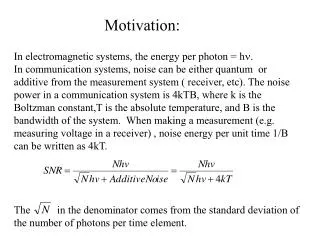
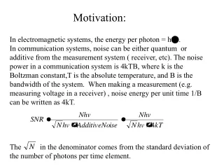
Motivation: In electromagnetic systems, the energy per photon = hn. In communication systems, noise can be either quantum or additive from the measurement system ( receiver, etc). The noise power in a communication system is 4kTB, where k is the Boltzman constant,T is the absolute temperature, and B is the bandwidth of the system. When making a measurement (e.g. measuring voltage in a receiver) , noise energy per unit time 1/B can be written as 4kT. The in the denominator comes from the standard deviation of the number of photons per time element.
Motivation: When the frequency n<< GHz, 4kT >> hn In the X-ray region where frequencies are on the order of 1019, hv >> 4kT So X-ray is quantum limited due to the discrete number of photons per pixel. We need to know the mean and variance of the random process that generate x-ray photons, absorb them, and record them. Recall: h = 6.63x10⁻³⁴ Js k = 1.38x10⁻²³ J/K
Motivation: Object we are trying to detect Contrast = ∆I / I SNR = ∆I / I = CI / I ∆I I Background We will be working towards describing the SNR of medical systems with the model above. We will consider our ability to detect some object ( here shown in blue)that has a different property, in this case attenuation, from the background ( shown here in green). To do so, we have to be able to describe the random processes that will cause the x-ray intensity to vary across the background.
1/6 1 2 3 4 5 6 The value of a rolled die is a random process. The outcome of rolling the die is a random variable of discrete values. Let’s call the random variable X. We write then that the probability of X being value n is px(n) = 1/6 Probability Note: Because the probability of all events is equal, we refer to this event as having a uniform probability distribution
Probability Density Function (pdf) 1/6 1 2 3 4 5 6 Probability Cumulative Probability Distribution 1 1 2 3 4 5 6
Continuous Random Variables pdf is derivative of cumulative density function p[x1≤ X ≤ x2] = F(x2) - F(x1) = 1. cdf is integral of pdf 2. cdf must be between 0 and 1 3. px(x) > 0
Zeroth Order Statistics • Not concerned with relationship between events along a random process • Just looks at one point in time or space • Mean of X, mX, or Expected Value of X, E[X] • Measures first moment of pX(x) • Variance of X, s2X , or E[(X-m)2 ] • Measure second moment of pX(x) Standard deviation
Zeroth Order Statistics • Recall E[X] • Variance of X or E[(X-m)2 ]
p(n) for throwing 2 die 6/36 5/36 Probability 4/36 3/36 2/36 1/36 7 12 2 3 4 5 6 8 9 10 11
Assumptions Fair die Each die is independent Let die 1 experiment result be x and called Random Variable X Let die 2 experiment result be y and called Random Variable Y With independence, pXY(x,y) = pX(x) pY (y) and E [xy] = ∫ ∫ xy pXY(x,y) dx dy = ∫ x pX(x) dx ∫ y pY(y) dy = E[X] E[Y] if x,y independent
Other helpful Theorems 1. E [X+Y] = E[X] + E[Y] Always 2. E[aX] = aE[X] Always 3. 2x = E[X2] – E2[X] Always 4. 2(aX) = a22x Always 5. E[X + c] = E[X] + c 6. Var(X + Y) = Var(X) + Var(Y) only if the X and Y are statistically independent. _
Binomial Random Variable If experiment has only 2 possible outcomes for each trial, we call it a Bernouli random variable. Success: Probability of one is p Failure: Probability of the other is 1 - p For n trials, P[X = i] is the probability of i successes in the n trials X is said to be a binomial variable with parameters (n,p)
Roll a die 10 times. In this game, you win if you roll a 6. Anything else - you lose What is P[X = 2], the probability you win twice? Example
Roll a die 10 times. 6 you win Anything else - you lose P[X = 2] i.e. you win twice = (10! / 8! 2!) (1/6)2 (5/6)8 = (90 / 2) (1/36) (5/6)8 = 0.2907 Example
If p is small and n large so that np is moderate, then an approximate (very good) probability is: p[X=i] is the probability exactly i events happen P[X=i] = e - i / i! Where np = Poisson Random Variable With Poisson random variables, their mean is equal to their variance! E[X] = sx2=
Let the probability that a letter on a page is misprinted is 1/1600. Let’s assume 800 characters per page. Find the probability of 1 error on the page. Binomial Random Variable Calculation. P [ X = 1] = (800! / 799!) (1/1600) (1599/1600)799 Very difficult to calculate some of the above terms. Example
Let the probability that a letter on a page is misprinted is 1/1600. Let’s assume 800 characters per page. Find the probability of 1 error on the page. P [ X = i] = e - i / i! Here i = 1, p = 1/1600 and n =800, so l=np = ½ So P[X=1] = 1/2 e –0.5 = .30 Example What is the probability there is more than one error per page? Hint: Can you determine the probability that no errors exist on the page?
Other Probability Density Functions + - Gaussian or Normal Random Variable
Other Poisson Random Variables Number of Supreme Court vacancies in a year 2) Number of dog biscuits sold in a store each day 3) Number of x-rays discharged off an anode
SNR (Signal to Noise Ratio) Signal Power Noise Power If X represents power, SNR = E[X]/ x2 If X represents an amplitude or a voltage, then X2 represents power. SNR = E[X]/ x
Screen Film Systems d X-ray photon Light photons x Film High density material stop photons through photoelectric absorption Scintillating material Screen creates light fluorescent photons. These get captured or trapped by silver bromide particles on film.
Analysis: First calculate spray of light photons from an event at depth x. r x h (r) = h(0) cos3 = h(0) x3 / (x2 + r2)3/2 Since h(0) = K/x2 K constant x2 inverse falloff h (r) = Kx / (x2 + r2)3/2
Analysis in Frequency Domain H1(r) = F{h(r)} ∞ = 2π ∫ h(r) J0 (2prr) r dr where h(r) given on previous page 0 H1(r) = 2πKe -2πxr (from a table Hankel transforms) H(r) = H1(r) = e -2πxr ( Normalize to DC Value) H1(0)
Analysis in Frequency Domain H(r) = H1(r) = e -2πxr ( Normalize to DC Value) H1(0) Notice this depends on x, depth of event into screen. Let’s come up with based on the likelihood of where events will occur in the scintillating material. F(x) = 1 - e - x for an infinite screen Probability an x-ray photon will interact in distance x F(x) x
p(x) = dF(x) / dx = e -x For a screen of thickness d F(x) = 1 - e -x / 1 - e -d , then since we are only concerned with captured photons H(p) = ∫ H(r,x) p(x) dx d = (1/ 1 - e -d )∫ e -2π x r e-x dx Typical d = .25 mm, m=15/cm for calcium tungstate screen
We would like to describe a figure of merit that would describe a cutoff spatial frequency, akin to the bandwidth of a lowpass filter. For a typical screen with d approximately .25 mm and m=15/cm for a calcium tungstate screen, the bracketed term above can be approximated as 1 for spatial frequencies near the cutoff.
Figure of Merit k 0.1 1.0 10 Cycles/mm rk For moderate k, (i.e. a cutoff frequency) Let (1 - e -d) = the capture efficiency of the screen Then k ≈ / (2πpk + ) 2πk pk = (1 - k) For k << 1 • : As the efficiency increases, rk decreases. This is because increases as d increases.
Dual Screen Systems d1 d2 phosphor phosphor x Double Emulsion film Intuitively, we would believe this system would work better . Let’s analyze its performance. Let d1 +d2 = d so we can compare performance.
H(r,x) = e -2πr (d1-x) for 0 < x < d1 H(r,x) = e -2πr (x –d1) for d1 < x < d1 + d2 d, d2 H(r) = (/ 1- e -d) { ∫ e -2πr (d1 - x) e - x dx + ∫ e -2πr (x –d1) e - x dx} 0 d1 = ( / 1- e -d) [ ((e -d1 - e -2πrd1) / (2πr - )) + ((e -d1 - e -(2πrd2 + d) / (2πr + u))] Again lets determine a cutoff frequency of rk for a low pass filter that has a response of H(rk) = k, If we assume d1 ≈ d2 = d/2, than we can neglect e -2πrd, e -2πrd1 , e -2πrd2 because they will be small even for relatively small spatial frequencies. e –ud is also small compared toe –ud1 Since (2πr)2 >> u2 istrue for all but lowest frequency, then
Compare this cutoff frequency to the single screen cutoff. Concentrate on the factor 2e-md1 ( the new factor from the single screen film) Since With h≈ 0.3, improvement is 1.7 Use improvement to lower dose, quicken exam, improve contrast, or some combination. Improvement is
Overall Response Assuming a circularly symmetric source, Id (xd, yd) = Kt (xd/M, yd/M) ** (1/m2) s (rd/m) ** h (rd) Detector response is also circularly symmetric.
Frequency Domain Id (u,v) = KM2T (Mu,Mv) S(mp) · H(p) H0(p) Spatial frequencies at detector Object is of interest though Id (u/M,v/M) = KM2T (u,v) S((m/M)p) · H(p/M) Product of 2 Low Pass Filters. H0(p) = S [(1-z/d) p ] H ((z/d)p)
As z d S(0) H(p) As z 0 H(0) S(p)