
Node Minimization
E N D
Presentation Transcript
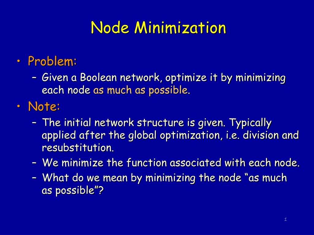
Node Minimization • Problem: • Given a Boolean network, optimize it by minimizing each node as much as possible. • Note: • The initial network structure is given. Typically applied after the global optimization, i.e. division and resubstitution. • We minimize the function associated with each node. • What do we mean by minimizing the node “as much as possible”?
Functions Implementable at a Node In a Boolean network, we may represent a node using the primary inputs {x1,.. xn} plus the intermediate variables {y1,.. ym}, as long as the network is acyclic. DEFINITION 1: A function gj , whose variables are a subset of {x1,.. xn,y1,.. ym}, is implementable at a node j if • the variables of gj do not intersect with TFOj • the replacement of the function associated with j by gj does not change the functionality of the network.
Functions Implementable at a Node • The set of implementable functions at j provides the solution space of the local optimization at node j. • TFOj = {node i s.t. i = j or path from j to i}
Prime and Irredundant Boolean Network Consider a sumofproducts expression Fj associated with a node j. Definition 2: Fj is prime (in multilevel sense) if for all cubes c Fj, no literal of c can be removed without changing the functionality of the network. Definition 3: Fj is irredundant if for all cubes c Fj, the removal of c from Fj changes the functionality of the network.
Prime and Irredundant Boolean Network Definition 4: A Booleannetwork is prime and irredundant if Fj is prime and irredundant for all j. Theorem 1: A network is 100% testable for single stuckat faults (sa0 or sa1) iff it is prime and irredundant.
Local Optimization Goals: Given a Boolean network, • make the network prime and irredundant. • for a given node of the network, find a least-cost sumofproducts expression among the implementable functions at the node. Note: • Goal 2 implies the goal 1, • But we want more than just 100% testability. There are many expressions that are prime and irredundant, just like in two-level minimization. We seek the best.
Local Optimization Key Ingredient Network Don't Cares: • External don't cares XDCk , k=1,…,p, - set of minterms of the primary inputs given for each primary output • Internal don't cares derived from the network structure • Satisfiability SDC • Observability ODC
SDC Recall: • We may represent a node using the primary inputs plus the intermediate variables. • The Boolean space is Bn+m . • However, the intermediate variables are dependent on the primary inputs. • Thus not all the minterms of Bn+m can occur.
SDC Example: y1 = F1 = x1 yj = Fj = y1x2 • Since y1 = x1, y1 x1 never occurs. • Thus we may include these points to represent Fj Don't Cares • SDC = (y1 x1)+(yj y1x2) In general, Note: SDC Bn+m
ODC yj = x1 x2 + x1x3 zk = x1 x2 + yjx2 + (yj x3) • Any minterm of x1 x2 + x2 x3 + x2 x3 determines zk independent of yj . • The ODC of yj for zk is the set of minterms of the primary inputs for which the value of yj is not observable at zk This means that the two Boolean networks, • one with yj forced to 0 and • one with yj forced to 1 compute the same value for zk when x ODCjk
Don't Cares for Node j Define the don't care sets DCj for a node j as ODC and SDC illustrated: outputs ODC Fj Boolean network S C D inputs
Main Theorem THEOREM 2: The function Fj = (Fj-DCj, DCj, Fj+DCj) is the complete set of implementable functions at node j COROLLARY 3: Fj is prime and irredundant (in the multi-level sense) iff it is prime and irredundant cover of Fj A leastcost expression at node j can be obtained by minimizing Fj. A prime and irredundant Boolean network can be obtained by using only 2level logic minimization for each node j with the don't care DCj . Note:If Fj is changed, then DCi may change for some other node i in the network.
Local Optimization Practical Questions • How to compute the don't care set at a node? • XDC is given, SDC is easy, • but how about ODC? • This don't care set may be too large. A good subset? • How to minimize the function with the don't care? • Complement may be too large? • #Literals v.s. #Cubes?
zk g1 gq g2 yj x1 x2 xn ODC Computation Denote where
zk g1 gq g2 yj x1 x2 xn ODC Computation In general,
ODC Computation Conjecture: This conjecture is true if there is no reconvergent fanout in TFOj. With reconvergence, the conjecture can be incorrect in two ways: • it does not compute the complete ODC. (can have correct results but conservative) • it contains care points. (leads to incorrect answer)
Transduction (Muroga-197x) Definition: Given a node j, a permissible function at j is a function of the primary inputs implementable at j. The original transduction computes a set of permissible functions for a NOR gate in an all NORgate network. MSPF (Maximum Set of Permissible Functions) CSPF (Compatible Set of Permissible Functions) Both of these are just incompletely specified functions, i.e. functions with don’t cares. Definition: We denote by gj the function fj expressed in terms of the primary inputs. • gj(x) is called the global function of j.
Transduction CSPF MSPF: • is expensive to compute. • if the function of j is changed, the MSPF for some other node i in the network may change. CSPF: • Consider a set of incompletely specified functions {fjC} for a set of nodes J such that a simultaneous replacement of the functions at all nodes jJ each by an arbitrary cover of fjC does not change the functionality of the network. • fjC is called a CSPF at j. The set {fjC} is called a compatible set of permissible functions (CSPFs).
Transduction CSPF Note: • CSPFs are defined for a set of nodes. • We don't need to recompute CSPF's if the function of other nodes in the set are changed according to their CSPFs • The CSPFs can be used independently. • Any CSPF at a node is a subset of the MSPF at the node • External don’t cares (XDC) must be compatible
Transduction CSPF Key Ideas: • Compute CSPF for one node at a time. • from the primary outputs to the primary inputs • If (f1C ,…, fj-1C )have been computed, compute fjC so that simultaneous replacement of the functions at the nodes preceding j by functions in (f1C ,…, fj-1C ) is valid. • put more don’t cares to those processed earlier • Compute CSPFs for edges so that Note: • CSPFs are dependent on the orderings of nodes/edges.
CSPF's for Edges Assume CSPF fiC for a node i is given. • Ordering of Edges: y1 < y2 < … < yr • put more don't cares on the edges processed earlier. • only for NOR gates 0 if fiC(x) = 1 f[j,i]C(x) = 1 if fiC(x) = 0 and for all yk > yj: gk(x) = 0 and gj(x) = 1 * (don’t care)otherwise
Transduction CSPF Example: y1 < y2 < y3 yi = [1 0 0 0 0 0 0 0] output y1 = [0 0 0 0 1 1 1 1] y2 = [0 0 1 1 0 0 1 1] y3 = [0 1 0 1 0 1 0 1] f[1,i]C = [0 * * * 1 * * *] f[2,i]C = [0 * 1 * * * 1 *] f[3,i]C = [0 1 * 1 * 1 * 1] Note: we just make the last 1 stay 1 and all others *. Note: CSPF for [1; i] has the most don't cares among the three input edges. i global functions of inputs edge CSPFs
CSPF Computation • Compute the global functions g for all the nodes. • For each primary output zk , fzkC(x)= * if xXDCk fzkC(x)= gzk(x) otherwise • For each node j in a topological order from the outputs, • compute fjC= iFOjf[j,i]C(x) • compute CSPF for each fanin edge of j, i.e. f [k,j]C [j,i] j [k,j]
Generalization of CSPF's A Boolean network where a node function is arbitrary (not just NOR gates). Based on the same idea as Transduction • process one node at a time in a topological order from the primary outputs. • compute a compatible don't care set for an edge, CODC[j,i] • intersect for all the fanout edges to compute a compatible don't care set for a node. CODCj= iFoj CODC[j,i]C • Put more don't cares on nodes/edges processed earlier.
Compatible Don't Cares at Edges Ordering of edges: y1 < y2 < … < yr • Assume no don't care at a node i. • A compatible don't care for an edge [j,i] is a function of CODC[j,i](y) : Br B Note: it is a function of the local inputs (y1 , y2 ,… ,yr). It is 1 at m Br if m is assigned to be don’t care for the input line [j,i].
yi no change i k j CODC[k,i](m)=1 CODC[j,i](m)=1 Compatible Don't Cares at Edges Property on {CODC[1,i],…,CODC[r,i]} • For all mBr, the value of yi does not change by arbitrarily flipping the values of { yjFIi | CODC[j,i](m) = 1 } m is held fixed, but value on yj can be arbitrary if CODC[j,i](m) is don’t care
Compatible Don't Cares at Edges Given {CODC[1,i],…,CODC[j-1,i]}compute CODC[j,i] (m) = 1 iff the the value of yi remains insensitiveto yj under arbitrarily flipping ofthe values of those yk in the set: = { kFIi | yk < yj, CODC[k,i](m) = 1 } Equivalently, CODC[j,i](m) = 1 iff for
Compatible Don't Cares at Edges (here ) Thus we are arbitrarily flipping the m part. In some sense is enough to keep fi insensitive to the value of yj. is called the Boolean difference of fi with respect to yj and is all conditions when fi is sensitive to the value of yj. • this is a function of FIi, but not yj.
Compatible Don't Cares at a Node Compatible don't care at a node j, CODCj, can also be expressed as a function of the primary inputs. • if j is a primary output, CODCj = XDCj • otherwise, • represent CODC[j,i] by the primary inputs for each fanout edge [j,i]. • CODCj= iFOj(CODCi+CODC[j,i]) THEOREM 7: The set of incompletely specified functions with the CODCs computed above for all the nodes provides a set of CSPFs for an arbitrary Boolean network.
Easier Computations of CODC Subset On page 46 of the paper by H. Savoj, an easier method for computing a CODC subset on each fanin ykof a function f is: where CODCf is the compatible don’t care already computed for node f, and where f has its inputs y1, y2 ,…, yr in that order. The notation for the operator, Cyf = fy fy , is used here.
Easier Computations of CODC Subset The interpretation of the term for CODCy2 is that: of the minterms mBr where f is insensitive to y2, we allow m to be a don’t care of y2 if • either m is not a don’t care for the y1 input or • no matter what value is chosen for y1, (Cy1), f is still insensitive to y2 under m (f is insensitive at m for both values of y2 )
Computing Don't Cares using BDD's Handles arbitrary Boolean networks. • MSPF's for general case • The complete set of implementable functions for a given node • incorporating SDC's
The Set of Implementable Functions Problem: Given a node j and a set of variables S { x1, …, xn, y1, …, ym }\TFOj, Find the set of all implementable functions for j, where the inputvariables of each function is a subset of S.
The Set of Implementable Functions Note: • SDC's are subsumed. • (S = {x1, …, xn} ) MSPF • (S = { x1, …, xn, y1, …, ym }\TFOj)the complete set of implementable functions at j.
The Set of Implementable Functions Definitions: gS : Bn B|S| the global functions of S;the ith function of gS is the global function of the ith variable of S. gZ : Bn { 0, 1, * }p the global functions of the primary outputs plus XDC zM : Bn+1 Bp the functions of the primary outputs expressed by the primary inputs and yj • for the node function of each primary output, recursively substitute each fanin by its node function, unless the fanin is either a primary input or yj j S
The Maximal Set of Implementable Functions Given S: Consider a Boolean relation FjM(s,yj) : B|S|B B s.t. xBn : (s = gS(x)) zM(x, yj) gZ(x) Note: FjM represents an incompletely specified function of s, i.e. if an s is associated with both yj = 1 and yj = 0 then yj = * (don't care for that s) Theorem 8: The set of functions given by FjM is the set of all implementable functions at j (as functions of the variables of S.) • Proof. Easy. j
BDD Computation for FjM(s,yj) • FjM(s,yj) is a relation a one to many map from syj • FjM(s,yj) 1 iff xBn : (s = gS(x)) zM(x,yj)gZ(x) Universal Quantification: For a function h : BrB of variables V={v1,v2,..,vr} and Vk ={v1,v2,..,vk} V, the universal quantification of h by Vk is the function hk of the variables V\Vk( = Vr- k ) s.t. hk(Vr-k) = 1 iff (VkBk ) h(Vk, Vr-k)=1. This is written as Vkh(v) of CVk h(v).
BDD Computation for FjM (s,yj) hk(Vr-k) = 1 iff (VkBk ) h(Vk, Vr-k)=1. hk is computed by successive cofactors of h by Vh. hk(Vr-k)=Cv1(Cv2(...Cvk(h)..)) where the operator The computation can be done easily using BDD's. Thus FjM can be computed and represented using BDD's.
The Set of Implementable Functions Remarks: • The BDD for FjM may be large. • Typically, S is set to FIjplus those variables whose fanins are a subset of FIj. • In processing y2 we use y3 since its support is a subset of the support of y2. • called the subset support filter. • corresponds to Boolean re-substitution since FjM is a function of y3.
Summary of Computation of Don't Cares • XDC is given, SDC is easy to compute. • Transduction • NORgate networks • MSPF, CSPF (permissible functions of PI only) • Extension of CSPF's (CODCs) for general networks • can be expensive to compute, not maximal • implementable functions of PI and y. • Direct computation using BDD's • the complete set of implementable functions • SDC's are also subsumed. • Subset of don't cares • TFIj and the nodes whose support are a subset of the fanins of j.
Minimizing Local Functions Once an incompletely specified function (ISF) is derived, we minimize it. 1. Minimize the number of literals • Minimum literal() in the slides for Boolean division 2. The offset of the function may be too large. • Reduced offset minimization (built into ESPRESSO in SIS) • Tautologybased minimization If all else fails, use ATPG techniques to remove redundancies.
Reduced Offset Idea: In expanding any single cube, only part of the offset is useful. This part is called the reduced offset for that cube. Example: In expanding the cubea b c the point abc isof no use. Therefore during this expansion abc might as well be put in the offset. Then the offset which was ab + ab + bc becomes a + b. The reduced offset is always unate. The trick is to derive the reduced offset for a particular cube without computing the offset.
Tautologybased TwoLevel Minimization In this, twolevel minimization is done without using the offset. Offset is used for blocking the expansion of a cube too far. The other method of expansion is based on tautology. Example: • In expanding a cube c = abeg to aeg we can test if aeg f +d. This can be done by testing (f +d)aeg 1 i.e. is (f + d) aeg a tautology?
ATPG MultiLevel Tautology: Idea: • Use testing methods. (ATPG is a highly developed technology). If we can prove that a fault is untestable, then the untestable signal can be set to a constant. • This is like expansion in espresso.
Removing Redundancies Redundancy removal: • do random testing to locate easy tests • apply new ATPG methods to prove testability of remaining faults. (if non-testable for s-a-1, set to 1 etc.) Reduction(redundancy addition) is the reverse of this. It is done to make something else untestable. There is a close analogy with reduction in espresso. Here also reduction is used to move away from a local minimum. & reduction = add an input d c a b used in transduction (Muroga) global flow (Bermen and Trevellan) redundancy addition and removal (Marek-Sadowska et. al.)
Multiple Output Functions Network of Multiple Output Functions: What is the set of implementable functions for fj at N? • Don't care formulation does not work • Boolean Relation: (completely specified) B : Bn2Bm (one to many mapping)
Multiple Output Functions Implementable functions: A function gj is an implementation (cover) of a Boolean relation B(gj p B )(or contained in) iff: x, gj(x)B (x)
Example: Boolean Relation Adder followed by comparator Want: f p B One solution: f = 000 if a + b 4,5,6 f = 100 if a + b = 4,5,6 This can’t be expressed with don’t cares