Logic Node Minimization for Combinational and Sequential Logic Synthesis
Minimization in logic node plays a crucial role in designing combinational and sequential logic circuits. This process optimizes behavior and flexibility while adhering to specified properties. By decomposing and optimizing the behavior, FSM synthesis is achieved. Node minimization addresses problems in FSM networks and optimization for permissible machine representations. Complex E-Machine calculations summarize permissible machines at a node. The logic E-Machine construction offers a solution to Problem 1, while fixed point calculation aids in finding optimal Mj for FSM nodes.

Logic Node Minimization for Combinational and Sequential Logic Synthesis
E N D
Presentation Transcript
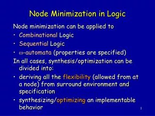
Node Minimization in Logic Node minimization can be applied to • Combinational Logic • Sequential Logic • -automata (properties are specified) In all cases, synthesis/optimization can be divided into: • deriving all the flexibility (allowed from at a node) from surround environment and specification • synthesizing/optimizing an implementable behavior
FSM FSM FSM FSM s2 a/1 s1 s3 a/0 Sequential Synthesis (Combinational logic and memory) • Computational Model • Network of interacting FSM’s (possibly cyclic) • FSM’s (general node) • Mealy or Moore • Symbolic/multi-valued (v has values in {stop, go, caution} ) • nondeterministic • several inputs and outputs per FSM node
FSM Specification FSM’s can be given by a state transition graph (STG): -0/01 inputs x, v outputs u,z 1-/11 2 x,v/u,z 00/10 -0/00 -1/10 1 start state 1 -1/01 3 01/10 or by a netlist of gates and latches (BLIF-MV format): latches Primary inputs Primary outputs
Sequential Synthesis • Decomposition/Collapsing collapsing = constructing product machine “Boolean” Division: Given two FSM’s M and M1, find FSM Q (quotient) such that M1 x Q = M. (What about M = M1 x Q + R )? • Node Minimization FSM FSM
Node Minimization: Two Problems Given: FSM Network and specification M : x z M Problem 1: Summarize and represent all permissible (implementable) machines at node j : Want : Sj such that Mj is permissible Mj Sj (i.e. Sj “simulates” Mj ) Past (partial) results: “don’t care” sequences • input (those that can’t occur) Kim and Newborn(1972) Devadas and Newton (1990) Somenzi (1991), Wang and Brayton (1993) • output ( pairs that can’t be distinguished) Problem 2: Find optimumMj , such is that Mj Sj if and only ifMj permissible.
The E-Machine (Watanabe ICCAD ‘93) Theorem: Given specification M : xz(in general a NDFSM) and FSM’s M1, M2, there exists a NDFSM E (called the E-machine) such that FSM N is permissible at M1NE E summarizes the Environment of M1
The E-Machine (Watanabe ICCAD ‘93) Ecan be computed by a (complicated ) fixed point calculation. NDFSM is represented using characteristic function of its transition relation: T (p,i,n,o ) = 1 Thus E summarizes all the permissible machines for M1 (solution to Problem 1)
Example E-machine for location M1: given given M2: M: specification u/v Note: do not need to know what M1 is
regular language S1S L automaton A FSM M E-machine Construction Using Logic S1S S1S stands for “Second order logic with 1Successor” Example: (describing a relation between sequence X and sequence Y). If a 1 appears at any even clock tick in X , a 1 also appears in Y at that time. Theorem: [Büchi 1961] A -language L is definable in S1S if and only if L is regular A language is regular accepted by an automaton
E-machine Construction Using Logic S1S Every FSM Mautomaton AM obtained by Accepting state Note: Every i/o is converted into io. Unspecified inputs transition to dummy node
S1S - Definitions & Background -Languages: Given finite set • *: set of all finite sequences over (random sequences) • A -language is a subset of * Notation: lower case variable (x) takes value in , upper case (X) in * Finite Automata (FA) 5-tuple (,S, s0,T,A) finite set called alphabet S finite set of states s0 S initial state T S x x S transition relation A S accepting states Deterministic FA: (s)(x)[ |{t : (s,x,t) T }| 1]; otherwise non-deterministic
Definitions & Background - II • String X * accepted by FA if there exists a sequence of states (a run) 0 1 ... nsuch that 1. n = |X|, 2. 0 = s0, n A, and 3. (i )[(i , Xi, i +1 ) T ] • Language of FA = set of strings accepted by it. • A -language is regular if it can be constructed by { x, ., +, , (, ) }, e.g. (a(b+c)).
Definitions & Background - II Facts: 1. Language is regular it is accepted by a DFA (If a NDFA, convert to DFA by power set construction) 2. Class of regular languages is closed under • Union, Intersection (product machine construction) • Projection (eraser construction) • Complementation (determinize with power set construction trivial complementation - exchange accepting and nonaccepting states).
Introduction & Background - III Logic S1S (second order theory of one successor): Natural logic for sets of sequences. • Formalism for describing properties of sequences; • powerful mechanism for analysis and manipulation of sequential systems (makes available full power of logic) Alphabet of S1S:{0,S,=,<,, ,,,x1,x2,…,X1,X2,…} (xi ) Syntax: • Terms: 0 | xi | St1 where t1 is a term. Examples: 0, SS0, SSSSx3. • Atomic formulae: t1 = t2 | t1 < t2 | t1 Xk where t1, t2 are terms, and Xk is a finite set of terms. Examples: (0 < S0), (x3 = SSSx5), (Sx7 X2 ) • S1S formulas: | () | (xi ) | (Xi ) where , are S1S formulae (including atomic formulae). Examples: (0 < S0) (Sx7 X2), (X )(x )[(x X )(Sx X )].
Introduction & Background - III S1S Semantics: Interpret over * = = {0,1,2,…}. Example 1:(Existence of least elements in non-empty subsets of ) = (X )[(x )(x X ) (y )((y X ) ((z)(z X (z < y ))))] Example 2:(Defining subsets of which contain 5 whenever they contain 3.) 0(X ) = (SSS0 X ) (SSSSS0 X ) Example 3:(Defining the subset of even integers) 1(X ) = (0 X ) (S0 X ) (x )(x X SSx X ) Example 4:(Defining the relation: “every even number is X is in Y” ) 2(X,Y ) = (x )[(Z )(1(Z ) x Z ) (x X x Y )] Given a formula (X1 ), the class of subsets of defined by (X1 ) is { | () is true}; Generally, formulae (X1,X2,…,Xn) define subsets of ( {0,1}n )*
Introduction & Background VI Obervation: Finite subsets of sequences over {0,1}. For example {0,2,3} is represented by 1011. We have to be careful about 0 sequences, e.g. to distinguish 00 from 000 etc. (Can do this by picking a length and extending each set to that length by putting 0’s at the end) Thus, S1S formulae define -languages. Theorem: [Büchi 1961] A -language is definable in S1S if and only if it is regular. 1-1
Advantages of S1S: Relationship between automata and S1S formally, succinctly express behaviors as formulae in S1S. In particular, • Automatic procedure for deriving automaton from formula. • Rigorous and constructive proofs for synthesis procedures.
The E-MACHINE-I Consider machines in configuration below. x, y observable inputs, outputs, LS (X x Y)* is a regular specification, i.e. the set of all (x, y) sequences in LS ((x1,y1),(x2,y2),…) is accepted by some automaton S.
The E-MACHINE-I Theorem: The set of all behaviors on u, v which will yield behavior on the inputs and outputs x, y compatible with the specification S (x,y) is given by the following S1S expression: E (V,U ) = (X,Y )[M (X,U,Y,V ) S (X,Y )] Proof: Convert each machine above to S1S expression. U,V,X,Y are sequences.
Constructing the E-Machinein Four Steps E (U,V ) = (X,Y )[M (X,Y,U,V ) S (X,Y )] = (X,Y )[M (X,Y,U,V ) S (X,Y )] can be rewritten in terms of manipulating automata: E (u,v ) = [(x,y )[M (x,y,u,v ) S (x, y )]] We use the correspondence between automata and FSM’s. Each of the operations in S1S, ,, corresponds to the automata constructions of product, complementation, and projection.
Constructing the E-Machine in 4 Steps Implies 4-step construction for E-machine E (u,v ) = [(x,y )[M (x,y,u,v ) S (x, y )]] 1. Complement the specification, S (x,y) S (x,y) 2. Form the product machine, P (x,y,u,v ) = M(x,y,u,v ) S (x,y ) 3. Existentially quantify out (erase) x,y from P, P (u,v ) = (x,y )[P (x,y,u,v )] 4. ComplementP, E (u,v ) = P (u,v ) ~ ~ ~
Comments on the Four Steps 1. S (x,y) S (x,y) If specification is non-deterministic, this may be exponential in |S| (number of states); a subset construction is required to complement S. 2. P (x,y,u,v) = M (x,y,u,v ) S (x,y) Easy; just the usual product machine construction. Using BDD’s, just multiply the two transition relations. 3. P (u,v ) = (x,y)[P (x,y,u,v )] Easy; existential quantification is simply a “hiding” of variables operation. In general quantifying variables leads to non-deterministic automata. ~
Comments on the Four Steps ~ 4. E (u,v) = P (u,v) If P (u,v) is non-deterministic, then potentially exponential; we have to determinize with the subset construction. However, the resulting automaton E is deterministic, and hence a “pseudo-nondeterministic” FSM. There are special cases (topologies), where the worst case behavior does not occur. ~ A pseudo-nondeterministic FSM is a nondeterministic FSM but whose automaton is deterministic.
Applications of the E-MACHINE Supervisory Control: Construct a controller C which controls a plant P so that it has a given behavior S. Rectification/Engineering Change: Modify an original design so that it conforms to a new specification S. • Note: These constructions have no quantification, • no introduction of non-determinism • if S is deterministic, then construction is polynomial.
The E-MACHINE II Cascade-I: y x u A1 A2 A 1(X,U ) = (Y )[ A 2(U,Y ) S (X,Y )] A 2(U,Y ) = (X )[ A 1(X,U ) S (X,Y )] Here, S (x,y) = (u)[A1(x,u) A2(u,y)], i.e. the specification is the currrent implementation. In this case, the machine A2* produced by the above construction is exactly that produced by the Kim and Newborn construction.
The E-MACHINE II Cascade-II: u v y x B1 B2 B3 B2(U,V ) = (X,Y )[B1(X,U ) B3(V,Y ) S(X,Y )] 2-way Cascade: u x y M1 M2 v M1(X,V,U ) = (Y )[ M2(V,U,Y ) S(X,Y )] M2(U,V,Y ) = (X )[ M1(X,V,U ) S(X,Y )]
Realizability The set LE defined by E(U,V ) is the set of all acceptable behaviors. In general, LE may not be realizable. This can happen in two ways. 1. There may be blocking input sequences V, i.e. sequences for which there is nooutputU such that (U,V ) LE. 2. A realization may not exist because of non-causality, viz the output may depend on future values of the input. Example: suppose (1,0),(1,1),(1,1),... Lbut (1,0),(1,1),(0,-),... L Thus, at the second step, the output can be 1 only if the next input is a 1. ~ ~ ~ ~
Realizability Definition 4:C is compatible with C * (CC *) provided that (V,U )[ C(V,U ) C*(V,U )] Realizability Problem: Given a regular LC*(V U)*, determine the existence of an implementable finite state machine C such that CC *. This can be solved by calling the following algorithm. ~ ~
Realizability Algorithm • Mealy algorithm: • Realizable_States: (DFAD: (SD, s0, VU, TD, AD)) • { • SC = SD, TC = TD, AC = AD; • while ( TRUE ) { • remove states s from SC, TC, AC such that • [(v )(u,t )[(s,v,u,t ) TC (t AC )] • if ( no states were removed ) • break; • } • return SC, TC, AC; • } Lemma 1:C * is realizableif and only if the set of states SC remaining after convergence contains the initial state. Further, there exists an implementable machine (completely specified, deterministic) C, CC * if and only if C C mealy, where C mealy is C * restricted to the states SC returned by the Mealy algorithm. ~ ~ ~
Moore Realizability Sometimes we want to restrict to Moore machines to ensure that there are no combinational cycles. • Moore algorithm: • Realizable_States: (DFAD: (SD, s0, VU, TD, AD)) • { • SC = SD, TC = TD, AC = AD; • while( TRUE ) { • remove statess from SC, TC, AC such that • [(v )(u )(t )[(s,v,u,t ) TC (t AC)] • remove transitionss,v,u,t from TCsuch that • [(s,v,u,t ) TC (v )(t )(s,v,u,t ) TC ] • if ( no states or transitions were removed ) • break; • } • return SC, TC, AC; • } ~ ~ ~ ~
Moore Realizability Lemma 2: 1. C * is realizable as a Moore machine if and only if the set of states SC remaining after the above Moore algorithm converges contains the initial state. 2. Further, there exists an implementable Moore machine (completely specified, deterministic),C, CC * if and only if C C moore, where C moore is C* restricted to the states SC returned by the Moore algorithm. However, even though there may not exist a Moore machine, there may exists a Mealy machine D Cmealy i.e. not all behaviors contained in Cmealy are Moore behaviors. ~ ~ ~
Problem 2 - Minimizing the node M1 Contained Behavior: E-Machine: Some contained behaviors: (deterministic FSM’s) contained in this:
E-machine is Pseudo Nondeterministic Definition 5: E = (U,V,S,T,r ) is a pseudo NDFSM(PNDFSM) if (sp,u,v) there exists at most one sn S such that T(sp,u,v,sn ) = 1, i.e. A E is deterministic. Thus when viewed as an automaton, a PNDFSM is deterministic: E-machine for M1 u is the input v is the output a=1/0 b=1/1 c=0/1 d=0/0 Deterministic Finite Automaton (incompletely specified)
Node Minimization One way to minimize a node in an FSM network is to “state minimize” the E-machine: Find a minimum state machine contained in E- machine. “State Minimization” Methods: Exact and heuristic methods exist for this. These use the notion of compatible sets of states generalized from incompletely specified machines to PSNDFSM. Watanabe - 1994 (exact and heuristic) Damiani - 1994 (exact) Kam and Villa - 1995 (exact method using implicit computation (BDDs) of compatibles).
FSM Node Minimization via ATPG(more practical) where O (E ) is the observability FSM of the E-machine E. O (E ) is a FSM obtained from E by converting each i /o pair to an input io, and completing it by adding a dummy state d, and an output, where output is 0 if io is a transition to d and 1 otherwise.
FSM Node Minimization via ATPG Since O (E ) is a completely specified FSM, we can implement it as a netlist and use sequential redundancy removal on M1. [H.Y. Wang - 1995].
Using Sequential Input Don’t Cares Before sequential ATPG is used we can transform the driving machine M2 by removing its inputs, simplifying and input determinizing (add new input(s) if machine is nondeterministic). Then sequential redundancy removal is used on the M1 part of the composed machine.
Summary - Sequential Synthesis Node minimization • know how to derive complete set of permissible behaviors (E- machine) • E-machine is a complex computation (possibly doubly exponential) but some topologies are easier. • exact and heuristic state minimizers for PNDFSM’s • use of sequential ATPG for minimizing given network relative to E-machine • limited right now to small machines • need more examples and experiments on use of approximate methods.
Design Verification and Refinement Problem: We want to verify that a given design satisfies a set of desired properties. Computational Model: • Network of NDFSM’s with fairness constraints. This models • system to be synthesized • its environment • Properties - expressed by either • -automata or • computational tree logic (CTL) with fairness constraints.
-Automata and Fairness Constraints Rabin: fair (acceptable) path r = (s0,s1,s2,…) is (F(Ui ) G(Vi )) where F(Ui ) inf(r) Ui G(Vi )) inf(r) Vi i Rabin Automaton With Rabin automata, one can express properties like infinitely often each time C requests service, eventually it gets access to service - a liveness property A Streett automaton is like a Rabin but with complementary fairness constraints: (F(Ui ) G(Vi )) i
Verification and Refinement Set of properties {P1,P2,…,Pn } acts like our system specification. Problems: 1. Summarize complete set of behaviors allowed locally at a single node, FSMj. 2. Refine(synthesize) a suitable implementation of FSMj (if one exists).
Generalized E-machine for Design Refinement P is desired property expressed as an -automaton. M2 is the rest of the system Restated as S1S Expression on Infinite Strings: Theorem 1:[Buchi (1960) ] A -language is expressible as an S1S expression if and only if it is -regular. Thus E (u,v) = (x,z)(M2(x,v,u,z ) P (x,z )) is an expression in S1S. Thus operationally, E (u,v) = (x,z )(M2 P ) exists. (It turns out thatE (u,v ) is a Rabin automaton.)
Generalized E-machine Construction E(u,v) = (x,z )(M2 P ) 1. Complement P. Generally, can express properties as deterministic Rabin automata (DR), so complementation into a deterministic Streett automata (DS), is easy. 2. FormM2 P. Easy since if M2 is Streett. 3. FormQ = (x,z)(M2 P ). Easy, but Q generally becomes NS. (Hiding variables generally causes nondeterminism). 4. Complement Q. We can do this by NS DR. The complexity is: NS (n,f ) DR (2 n2 log(n2 ) ) where n is the number of states and f the number of fairness constraints (Saffra - 1988). This has been implemented (Tasiran & Hojati). f f
Summary - Design Refinment In theory, we have a solution to the problem of finding all permissible behaviors when our initial specification is a set of properties. (Note: the construction is hierarchical ).
The Ultimate Synthesis Problem Open Questions: • how to find a contained behavior in E-automaton, i.e. a completely specified deterministic FSM. • how to find a minimum contained behavior
Conclusions • Common theme: for synthesis of combinational, sequential, and -automata for the node minimization problem. • Problems of synthesis and verification are closely related in all three areas. • Common model: network of automata.

