Routing Algorithms
Routing Algorithms. Tahir Azim. Outline . Overview of Routing in the Internet Hierarchy and Autonomous Systems Algorithms Naïve: Flooding Distance vector: Distributed Bellman Ford Algorithm Link state: Dijkstra’s Shortest Path First-based Algorithm Interior and Exterior Routing Protocols

Routing Algorithms
E N D
Presentation Transcript
Routing Algorithms Tahir Azim Courtesy: Nick McKeown, Stanford
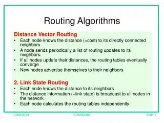
Outline Overview of Routing in the Internet • Hierarchy and Autonomous Systems Algorithms • Naïve: Flooding • Distance vector: Distributed Bellman Ford Algorithm • Link state: Dijkstra’s Shortest Path First-based Algorithm Interior and Exterior Routing Protocols • Interior Routing Protocols: RIP, OSPF • Exterior Routing Protocol: BGP Multicast Routing Routing is a very complex subject, and has many aspects. Here, we will concentrate on the basics. Courtesy: Nick McKeown, Stanford
The Problem “B” “A” R2 R1 R4 R3 How does R1 choose a next-hop on the path towards host B? Courtesy: Nick McKeown, Stanford
Metrics Delay to send an average size packet (Make high speed links attractive, but closeness counts) Bandwidth Link utilization Stability: Is a link (or path) up or down? Today: about 1/3 of Internet routes are asymmetric Routing Metrics Courtesy: Nick McKeown, Stanford
Example network Objective: Determine the route from A to B that minimizes the path cost. Examples of link cost: Distance, data rate, price, congestion/delay, … A 1 1 4 R1 R2 R4 R6 2 3 2 2 R7 3 R5 2 R3 4 R8 B Courtesy: Nick McKeown, Stanford
Example network In this simple case, solution is clear from inspection A 1 1 4 R1 R2 R4 R6 2 3 2 2 R7 3 R5 2 R3 4 R8 B Courtesy: Nick McKeown, Stanford
So what about this network...!?The public Internet in 1999 Learn more at http://www.lumeta.com Courtesy: Nick McKeown, Stanford
Routing in the Internet The Internet uses hierarchical routing • The Internet is split into Autonomous Systems (AS’s) • Examples of AS’s: Stanford (32), HP (71), MCI Worldcom (17373) • Try:whois –h whois.arin.net “MCI Worldcom” • Within an AS, the administrator chooses an Interior Gateway Protocol (IGP) • Examples of IGPs: RIP (rfc 1058), OSPF (rfc 1247). • Between AS’s, the Internet uses an Exterior Gateway Protocol • AS’s today use the Border Gateway Protocol, BGP-4 (rfc 1771) Courtesy: Nick McKeown, Stanford
Routing in the Internet AS ‘B’ AS ‘A’ AS ‘C’ BGP BGP Interior Gateway Protocol Interior Gateway Protocol Interior Gateway Protocol Stub AS Transit AS e.g. backbone service provider Stub AS Courtesy: Nick McKeown, Stanford
Routing Algorithms Courtesy: Nick McKeown, Stanford
R1 Technique 1: Naïve Approach Flood! -- Routers forward packets to all ports except the ingress port. • Advantages: • Simple. • Every destination in the network is reachable. • Disadvantages: • Some routers receive a packet multiple times. • Packets can go round in loops as long as TTL>0. • Inefficient. Courtesy: Nick McKeown, Stanford
Spanning Trees Objective: Find the lowest cost route from each of (R1, …, R7) to R8. 1 1 4 R1 R2 R4 R6 2 3 2 2 R7 3 R5 2 R3 4 R8 Courtesy: Nick McKeown, Stanford
A Spanning Tree 1 1 4 R1 R2 R4 R6 3 2 2 2 R7 R5 2 3 4 R3 R8 • The solution is a spanning treewith R8 as the root of the tree. • Tree: There are no loops. • Spanning: All nodes included. • We’ll see two algorithms that build spanning trees automatically: • The distributed Bellman-Ford algorithm • Dijkstra’s shortest path first algorithm Courtesy: Nick McKeown, Stanford
Technique 2: Distance VectorThe Distributed Bellman-Ford Algorithm , for all i, to This is the “Distance vector”. Courtesy: Nick McKeown, Stanford
2 4 1 1 R4 R6 R1 R2 3 2 2 3 2 2 R7 3 R5 2 4 R8 4 R3 Bellman-Ford Algorithm Example 1 1 4 R1 R2 R4 R6 2 3 2 2 R7 3 R5 2 R3 4 R8 Courtesy: Nick McKeown, Stanford
Solution 5 4 5 2 1 1 R1 R2 R4 R6 2 3 2 2 R7 3 4 R5 2 R3 R8 4 Bellman-Ford Algorithm 6 4 6 2 1 1 4 R1 R2 R4 R6 3 2 3 2 2 2 R7 3 4 R5 2 4 R3 R8 Courtesy: Nick McKeown, Stanford
Bellman-Ford Algorithm Questions: • How long can the algorithm take to run? • How do we know that the algorithm always converges? • What happens when link costs change, or when routers/links fail? Topology changes make life hard for the Bellman-Ford algorithm… Courtesy: Nick McKeown, Stanford
A Problem with Bellman-Ford “Bad news travels slowly” 1 1 1 R1 R2 R3 R4 Consider the calculation of distances to R4: Time R1 R2 R3 R3 R4 fails 0 3,R2 2,R3 1, R4 1 3,R2 2,R3 3,R2 2 3,R2 4,R3 3,R2 3 5,R2 4,R3 5,R2 … … … … “Counting to infinity” Courtesy: Nick McKeown, Stanford
Set infinity = “some small integer” (e.g. 16). Stop when count = 16. Split Horizon: Because R2 received lowest cost path from R3, it does not advertise cost to R3 Split-horizon with poison reverse: R2 advertises infinity to R3 There are many problems with (and fixes for) the Bellman-Ford algorithm. Counting to Infinity ProblemSolutions Courtesy: Nick McKeown, Stanford
Routers send out update messages whenever the state of an incident link changes. Called “Link State Updates” Link State Updates are flooded throughout the network Based on all link state updates received each router calculates lowest cost path to all others, starting from itself. Use Dijkstra’s single-source shortest path algorithm Assume all updates are consistent At each step of the algorithm, router adds the next shortest (i.e. lowest-cost) path to the tree. Finds spanning tree rooted at the router. Technique 3: Link StateDijkstra’s Shortest Path First Algorithm Courtesy: Nick McKeown, Stanford
The Link State Packet: The ID of the router that created the LSP List of directly connected neighbors and cost to each neighbor Sequence number TTL Reliable Flooding Resend LSP over all links other than incident link, if the sequence number is newer. Otherwise drop it. Link State Detection: Link layer failure Loss of “hello” packets Reliable Flooding of LSP Courtesy: Nick McKeown, Stanford
Example network (seen before) Objective: Determine the route from A to B that minimizes the path cost. A 1 1 4 R1 R2 R4 R6 2 3 2 2 R7 3 R5 2 R3 4 R8 B Courtesy: Nick McKeown, Stanford
Dijkstra’s Shortest Path First AlgorithmExample R5 2 R8 R6 2 R5 R8 2 R6 R7 2 3 R5 R8 2 Courtesy: Nick McKeown, Stanford
Dijkstra’s Shortest Path First AlgorithmExample Courtesy: Nick McKeown, Stanford
Dijkstra’s SPF Algorithm 1 1 R1 R2 R4 R6 2 2 R7 3 R5 2 R8 R3 4 Courtesy: Nick McKeown, Stanford
Distance Vector vs Link State • Messages • Size: small with LS; potentially large with DV • Exchange: LS flood!; DV only to neighbors • Space requirements • LS maintains entire topology • DV maintains only neighbor state • Robustness: • LS can broadcast incorrect/corrupted LSP • Can be made robust since sources are aware of alternate paths • DV can advertise incorrect paths to all destinations • Incorrect calculation can spread to entire network • Examples (coming up later): • LS: OSPF • DV: RIP, RIP2 Courtesy: Nick McKeown, Stanford