Routing algorithms
Routing algorithms. Routing algorithms establish the path followed by each message or packet. Routing algorithms for wormhole routing are also valid for other switching techniques.

Routing algorithms
E N D
Presentation Transcript
Routing algorithms • Routing algorithms establish the path followed by each message or packet. • Routing algorithms for wormhole routing are also valid for other switching techniques. • Routing algorithms can be classified according several criteria, such as adaptivity, progressiveness and minimality. NC2 (No.5)
Taxonomy of routing algorithms Routing algorithms Unicast Routing multicast Routing source Routing distributed (incremental) Routing Routing table lookup Finite-state machine (algorithmic routing) NC2 (No.5)
Adaptivity (1/2) • Deterministic routing algorithm always supply the same path between a given source / destination pair. • Adaptive routing algorithms use information about network traffic and/or channel status to avoid congested or faulty regions. • Adaptive routing can be classified as progressive or backtracking. NC2 (No.5)
Adaptivity (2/2) • Minimal (profitable) or nonminimal: Forward packets closer to their destination or not • Fully adaptive or partially adaptive: All the packets can be adaptively routable, or A part of the set of packets (e.g. classified by their destination) can be adaptively routed, and the rest of them cannot. • In practical, adaptive routing can be beaten by deterministic algorithms on some metrics. NC2 (No.5)
Source routing (1/2) • The source node specifies the routing path on the basis of a deadlock-free routing algorithm. • The computed path is stored in the packet header, being used at intermediate nodes to reserve channels. • It has been mainly used in computer networks with irregular topologies (e.g. Myrinet). NC2 (No.5)
Source routing (2/2) • When the long header is transmitted through the network, it comsumes network bandwidth. • Because the shorter header is preferable, street-sign routing uses the header contains only the node address at which the turn will take place and the direction of the turn (e.g. iWarp). NC2 (No.5)
Source routing (examples) d e f c a b Naive source routing b c d e f Street-sign routing b(upper) d(right) Output port encoding E N N E E X NC2 (No.5)
Distributed routing • A path of a packet is determined in a distributed manner while the packet travels across the network. • For efficiency reasons, most hardware routers use distributed routing. • The header requires the destination address and a few implementation-dependent control bits (very compact). NC2 (No.5)
Table-lookup routing • A routing table, which contains the number of entries equal to the number of nodes in the network, is placed at each node. • In the case of source routing, a table entry indicates the whole path to reach the destination node. • In the distributed routing, each table entry indicates which outgoing channel should be used to forward the packet toward its destination. (e.g. interval routing in Inmos T9000 transputer and its router C104) NC2 (No.5)
Node-Table routing • Table-based routing can be performed by storing the routing table in the routing nodes rather than the terminals. • Node-table routing is more appropriate for adaptive routings because it enables the use of per-hop network state information to select among several possible next hops at each stage of the route. • Performing a lookup at every step of the route, rather than just at the source, significantly increases the latency for a packet to pass through the router. NC2 (No.5)
Interval routing Y+ 0 4 8 12 Routing table for node 5 X+ 8-15 X- 0-3 Y+ 4 Y- 6-7 1 5 9 13 2 6 10 14 3 7 11 15 Y- X- X+ NC2 (No.5)
Finite-state machine routing • Most parallel computers use topologies that can be decomposed into orthogonal dimensions (e.g. mesh, hypercube tree). • In these topologies, it is possible to use simple routing algorithms based on finite-state machines. • For example, dimension-order routing routes packets by crossing dimensions in increasing order, nullifying the offset in one dimension before routing in the next one. • Such algorithmic routing is often more efficient in terms of both area and speed than table-based routing. NC2 (No.5)
Dimension-order routing(e-cube routing) Y+ 0 1 2 3 4 5 6 7 8 9 10 11 12 13 14 15 Y- X- X+ NC2 (No.5)
Deterministic ruoting • It always provides the same output channel for the same destination. • Routing decision is independent of (i.e. oblivious to) the state of the network. • It became popular when wormhole switching (compact and fast hardware router is desirable) was invented. NC2 (No.5)
X-Y routing for 2-D meshes Inputs: coordinates of current node (Xc, Yc) destination node (Xd, Yd) Xo=Xd-Xc; Yo=Yd-Yc; If Xo<0 then channel=X-; If Xo>0 then channel=X+; If Xo=0 and Yo<0 then channel=Y-; If Xo=0 and Yo>0 then channel=Y+; If Xo=0 and Yo=0 then channel= internal; NC2 (No.5)
E-cube routing for hypercube (1/2) Inputs: addresses of current node current and destination Dest Offset = current^ Dest; If Offset = 0 then channel = internal; Else channel = firstOne(Offset); where firstOne(Offset) returns the position of the first bit set to one NC2 (No.5)
E-cube routing for hypercube (2/2) 1111 1110 0111 0110 1010 0010 0011 1100 0101 0100 1101 1001 0001 0000 1001 0000 →0001 →0011 → 0111 →1111 NC2 (No.5)
Dimension-order routing for unidirectionial 2-D tori (1/2) C00 00 10 20 C01 C11 01 11 21 C10 02 12 22 NC2 (No.5)
Dimension-order routing for unidirectionial 2-D tori (2/2) Inputs: coordinates of current node (Xc, Yc) destination node (Xd, Yd) Xo=Xd-Xc; Yo=Yd-Yc; If Xo<0 then channel=C00; If Xo>0 then channel=C01; If Xo=0 and Yo<0 then channel=C10; If Xo=0 and Yo>0 then channel=C11; If Xo=0 and Yo=0 then channel= internal; NC2 (No.5)
Partially adaptive routing • Partially adaptive routing represent a trade-off between flexibility and cost. • Try to approach the flexibility of fully adaptive routing at the expense of a moderate increase in complexity with respect to deterministic routing. • Most of them rely upon the absence of cyclic dependencies between channels to avoid deadlock. NC2 (No.5)
Planar-adaptive routing (1/2) • One of the partially adaptive routing for n-dimensional meshes and hyperecubes[Chien and Kim]. • It provides adaptivity in only two dimension at a time. • A packet is routed adaptively in a series of 2-D planes. NC2 (No.5)
Planer-adaptive routing (2/2) destination A2 A1 A1 A1 A0 A0 A0 source Fully adaptive Planar-adaptive NC2 (No.5)
Turn model (1/3) • It is the minimal or nonminimal partially adaptive routing[Glass and Ni,1992]. • It prohibits the turns that form a cycle. • Deadlock cab be avoided by prohibiting just enough turns to break all the cycles. NC2 (No.5)
Turn model (2/3) North-last west-fast Negative-first X-Y dimension-order NC2 (No.5)
Turn model (3/3) X X X X X X X NC2 (No.5)
Fully adaptive routing • A fully adaptive routing algorithms can use all the physical paths from source to destination. • It may restrict the use of virtual channels to avoid deadlock. • Some deadlock recovery algorithms have no restriction on the use of virtual channels (true fully adaptive). NC2 (No.5)
Hop algorithms • Gopal proposed several fully adaptive minimal routing algorithms which are known as hop algorithms[Gopal,1985]. • They use structured buffer pools to avoid deadlock. • If the network diameter is D, a minimum of D+1 buffers per node are required. • A packet in a buffer class i will be stored in a buffer class i+1 in the next node (positive-hop algorithm). NC2 (No.5)
Structured buffer pool (1/2) node0 node1 node2 node3 Positive-hop Label 0 Label 1 Label 0 Label 1 negative-hop NC2 (No.5)
Structured buffer pool (2/2) • Structured buffer pool was designed for store-and-forwarding networks using central buffers. • Replacing the central buffers by virtual channels, the hop algorithms can suit for wormhole switching. • Resulting algorithms can be fully adaptive minimal routing for any topology at the expense of high number of virtual channels. NC2 (No.5)
Virtual channel balance • A hop algorithm produces an unbalanced use of virtual channels because all the packets start from virtual channel 0, however few packets take the maximum number of hops. • It can be improved by giving each packet a number of bonus cards (MAX hops – actual hops). • At each node, a packet has some flexibility, the range of virtual channels equal to the bonus cards+1, in the selection of virtual channels. NC2 (No.5)
Virtual networks • A network is split into several virtual networks using virtual channels (VCs). • They are disjoint channels sets. • Each virtual network can be defined in such a way that the corresponding routing function has no cyclic dependencies between channels. • Packets transfers between virtual networks are restricted in such a way that deadlock is avoided. NC2 (No.5)
Linder and Harden’s adaptive algorithm • Split n-dimensional meshes into 2n-1 virtual networks. • Each virtual network has channels in both directions in the 0th dimension and only one direction in the remaining n-1 dimensions. • The number of VCs across each physical channel is 2n-1, except for dimension 0 which has 2n. NC2 (No.5)
Virtual networks for a 2-D mesh 0 1 2 3 0 1 2 3 4 5 6 7 4 5 6 7 8 9 a b 8 9 a b c d e f c d e f Virtual network 0 Virtual network 1 NC2 (No.5)
Turns allowed on each virtual network Virtual network 0 Virtual network 1 It is called double-x routing. NC2 (No.5)
Duato’s protocol (1/4) • Duato proposed design methodologies for fully adaptive routing [Duato, 1991]. • They usually supply near-optimal minimal or nonminimal routing algorithms. • When restricted to minimal paths, the resulting algorithms are referred as Duato’s protocol (DP). NC2 (No.5)
Duato’s protocol (2/4) • For an interconnection network I, select one of the existing routing functions R1. It must be deadlock-free and connected. It can be deterministic or adaptive. Let C1 be the set of channels for R1. • Split each physical channel into a set of additional VCs. Let C be the set of all the VCs. Define the new routing function as; R(x,y) = R1(x,y)∪(Cxy∩(C-C1), where Cxy is the set of output channels from node x to node y NC2 (No.5)
Duato’s protocol (3/4) • R(x,y) is the new routing function which can use any of the new channels or, alteratively, the channels supplied by R1. • For wormhole switching, verify that the extended channel dependency graph for R1 is acyclic. If it is, the routing function is valid. Otherwise, it must be discarded, returning to step 1. NC2 (No.5)
Duato’s protocol (4/4) • For step 1, deterministic or turn model should be preferred for R1. • Step 2 indicates how to add more VCs to the network and how to define a new fully adaptive routing function. • The last verification step is not required for VCT and SAF, but it is only required for wormhole switching. Many minimal functions pass this step, but few nonminimal functions pass it. NC2 (No.5)
An example of DP (1/2) • For 2-D mesh using SAF, select XY dimension-order routing as R1. • Split each physical channel ci into ai and bi. • Let C1 be the set of bi channels (C-C1=ai). • R supplies all the outgoing ai channels from the current node, also supplying one b channel according to dimension-order routing. • When restricted to minimal paths, R is also deadlock-free for wormhole switching. NC2 (No.5)
An example of DP (2/2) a 0 1 2 3 b b a 4 5 6 7 8 9 a b c d e f NC2 (No.5)
History (routing) • Early networks performed routing in software. • For example, processors explicitly relay communications in the Solomon machine (1962). • By the mid-1980s, router chips, such as for tori, were developed. • Those routers forward messages throw networks without processor intervention. • Today, the software switching that requires terminal’s resources is rarely used. NC2 (No.5)
History (adaptive routing) • Many adaptive routing algorithms give poor worst-case performance because they use only local network state resulting in global imbalance. • Duato’s protocol enabled a family of adaptive routing algorithms including the one used in Cray T3E and IBM Bluegene/L. • Minimal adaptive routing on a fat tree was used in the CM-5 and Quadrics Q’sNet. NC2 (No.5)
History ( deadlock-prevention) • Early work on deadlock-free interconnection networks identified the technique of enumerating network resources and traversing these resources an increasing order. • Linder and Harden developed a method that makes arbitrary adaptive routing deadlock-free but at the cost of a number of virtual channels (1991). • Duato’s protocol has been used in several networks such as Cray T3E and the Alpha 21364. NC2 (No.5)
Bibliographic notes • Table-based source routing is popular in implementation due to its flexibility (ex. IBM SP1 and SP2). • Larger networks, such as SGI Spider, Infiniband, and the Internet, adopt node-tables to reduce the table size. • Hierarchical routing and interval routing are also the approaches for reducing table size. • CAMs are common in the implementation of routing tables. NC2 (No.5)