Download
1 / 57
570 likes | 591 Vues
Explore the real options in energy finance with a focus on infrastructure and commodity analysis. Learn about estimating costs, discounted cash flows, and commodity finance tools. Dive into Corn Ethanol plant models and gain insights into energy finance.

E N D
Real Options in Energy Finance Matt Davison,Professor of Applied Mathematics and Statistical & Actuarial Sciences Dean of Science, Western University Canada, London Ontario BIRS Thursday Sept 26 2019
Collaborators • Matt Thompson (Queens Business School) • Lindsay Anderson (Cornell University) • Guangzhi Zhao (Royal Bank) • Natasha Burke (née Kirby), (TD Bank) • Walid Mnif (TD Bank) • Christian Maxwell(Bank of Montreal) • Behzad Ghafouri(entrepreneur) • Nicolas Merener, Dean of Business, Universidad Torcuata di Tella, Buenos Aires, Argentina • Somayeh Moazeni, Stevens Institute of Technology • Junhe Chen (Current Western PhD student)
The Canadian Economy in 2017 • Canada has world leading companies in banking, insurance, and mining • (Data StatsCan)
Infrastructure can “create” a commodity or “transform” it “Create” • Hydro dam • Wind Turbine • Copper Mine “Transform” • Corn Ethanol Plant • Coal power plant • Gas power plant
Need expensive, long-lived infrastructure Expensive • LNG terminal in Kitimat BC cost $40BB to build • Wind turbine $2MM to build each– and farm has 50-100 Long Lived • Bruce power plant first begun in 1970 • Parts of the Niagara Falls Beck power plant were built in the 1920s in about their current form
Risks Commodity Finance Must Solve • Price Risk • Supply Risk • Demand Risk • Regulatory Risk • Geopolitical Risk • Technological Risk • Hedging • Insurance • Storage • + Operational Flexibility for all categories!
Questions Value infrastructure? • The Value of a piece of infrastructure is the value of the infrastructure when optimally operated Operate Infrastructure? • This depends on the value of plant, as we shall see • This circularity and the corresponding nonlinearity is nothing new in quant finance!
Real Business Decisions Discounted Cash Flow Real Options But projects may have optionality. For instance, if project works, it may have long sequence of profitable years If it doesn’t work it can be cancelled Looks like an option • Estimate all costs and incomes from a given project • In each year, net cash flow is Income – Costs • Discount cash flows by “hurdle rate”: higher uncertainty, higher hurdle rate • If DCF > 0 proceed, otherwise do not
Commodity Finance • Uses many of the same tools as regular quantitative finance • Emphasis on spreads: Calendar, location, spark/dark/crush spreads • Real things with real physical properties implement these spreads. • Political risk and government subsidies key • Often regional in nature with oligopolistic structure.
Corn Ethanol • Schmitt and his colleagues at Cornell • Gonzalez et al. 2013 • Schmitt & Luo (Energy Economics 2011) • N. Kirby & MD (2010). Energy Economics • C. Maxwell & MD (2014). Energy Economics42, pp. 140-151 • C. Maxwell & MD (2015). In Commodities, Energy, and Environmental Finance. M. Ludkowski,
Ethanol • (Corn) ethanol biofuel production in North America has become popular • Encouraged by government subsidies (“green”, “safe”, also good politics). • Market is fairly easy to understand, model, and quantify • Looking at ethanol gives insights about energy finance in general.
Corn model • Corn + nat gas Ethanol + Distiller’s dried grains • Very simple model: net the grains out to get • 1.25 bushels of corn 1 gallon of ethanol
Simple example • Model spread yt as very simple arithmetic Brownian motion • dyt = bdWt (no drift); Wt a Wiener process • If spread is positive, run the plant and get one gallon of gasoline per time unit • If spread is negative, idle the plant • Assume plant lasts forever • Don’t worry, we’ll relax all these crazy assumptions later. This is just for insight
Value integral • Value depends on spread and state and time • V0(y) is value if off and spread is y (y < 0) • V1(y) is value if on and spread is y V= max(V0,V1) V = E{∫t∞ f(ys)exp[-r(s-t)]ds} f(ys) = max(ys,0) V’(∞) = 1/r; V(-∞) = 0
ODE • V(y,t) = (1-rdt)V(y+dy,t+dt) + f(y)dt • -rVdt + V(y+dy,t+dt)-V(y,t) + f(y)dt • Cancel higher order terms and use Ito: • -rVdt + E{bV’(y)dW + ½ b2 V’’(y)dt} + f(y)dt • E{dW} = 0 and cancel dt’s to get: • -rV(y) + ½ b2 V’’(y) + f(y) = 0 • This holds both for on and off states so:
Two ODEs y < 0 ½b2V0’’(y) - rV0 = 0 V0(-∞) = 0 Smooth pasting y > 0 ½b2V1’’(y) - rV1 + y = 0 V1’(∞) = 1/r • V0(0) = V1(0) • V0’(0) = V1’(0)
Solution • Eigenvalues +/- √(2r)/b • Very simple ODE problem to find: • V0(y) = b/(2r)1.5 exp[√(2r)y/b] • V1(y) = b/(2r)1.5 exp[-√(2r)y/b] + y/r
You just blew my mind! • dy = bdW; b is risk • More risk to price, more value to plant! • Makes sense… • But mind bending to traditional thinkers • See Lehmberg & Davison 2014
Stuff we ignored • Spread really not simple ABM • Costs money to turn plant on and off • Inputs can include government subsidies: time varying and to some degree unpredictable • {Subsidies not just explicit but also implicit through regulations – current work with Merener not discussed today}
My research program for past decade • Look at real options model of corn ethanol plant with successively more realism • Real Options model including realistic cost structure • Including stochastic subsidy model • Considering bigger complexity of rules (not just money: ethanol mandate and blending wall
The Ethanol Market in the USA • 209 plants produced 13.3 billion gallons in 2012 • Subsidies a big part of this: Began with $0.40 per gallon in 1978 (Energy Tax Act) and then changed a lot over time; subsidies expired in 2012.
Empirical impact of subsidy change • In 2013 about ¼ of Nebraska’s energy plants were idle • Loss of subsidies are a possible contributing factor as many suggest that corn ethanol is not sustainable without subsidies. • We use a real options analysis to discover how plants will be operated knowing that subsidies may change.
Mini Outline 1. Plant Characteristics, Management Decisions, Associated costs and profits 2. Stochastic Optimal Control for optimal plant operating rule/plant value 3. Numerical Results & Policy Conclusions
What is the real option?: • Run plant when ethanol is worth more than cost of inputs; idle plant when it is not • There are switching costs between “on” and “off” –, this will lead to hysteresis
Assembling the model • A model for policy impact on ethanol production requires: • A model for the plant including flexibility of control, capitalized construction costs, profit as a function of ethanol/corn prices, costs to pause/resume production • Stochastic models for corn & ethanol prices and for subsidy level • Optimal operating rule which maximizes future profits
Management Flexibility • Management can: • Start/Stop production to avoid running at a loss over sustained periods or to recapture profits if price spread becomes favourable again • Two main states: on (1), off (0). • Turn production “on” from “off”: penalty $D01 per gallon • Turn production “off” from “on”: penalty $D10 per gallon
Profit functions • In regime i running profit is fi(…) • Corn ethanol + by-products • Yield (gallons ethanol/bushel corn): κ • Ethanol $Lt/gallon; Corn $Ct (/bushel) • Subsidy: $Zt/gallon • Running costs = $K1/gallon; Idle cost $K0 • So f1 = κ(Lt+ Zt - K1)-Ct • Also f0 = -κ(K0)
Stochastic Subsidy Model • Model stochastic subsidy by pure Poisson jump process with • arrival rate λ • jumps of size J (lognormally distributed with parameters α and β) • dZt = (J-Zt)dNt • Nt is a counting process for which dNt = 1 with probability λdt and 0 otherwise.
The Moving Boundary PDE • Either it is optimal to stay in the current state i, in which case this PDE is satisfied: δVi/δt + L[Vi] + I[V] + fi(t,L,C,Z) – rVi = 0, Vi ≥ Vj – Dij • Or it is optimal to switch in which case: Vi(t,L,C,Z) = Vj(t,L,C,Z) – Dij
Qualitative Results (1) • This implies the more uncertainty about subsidies (and prices) the better. • This arises from the ability to react to uncertainty by idling the plant • We can hedge price uncertainty, not subsidy uncertainty. • This makes the uncertainty in knowing the parameters of the subsidy uncertainty critical
Uncertainty Aversion: same PIDE • With different parameters for bid/offer price: • Theorem (Worst case Price) The option price is bounded above by the worst case price for which α = αmin • and λ = λmin if E[V(l,c,z+J)]-V(l,c,z) >= 0; otherwise λ = λmax. • Similar result holds for best-case price.
Simplified model • Look at “stripped down” model where we model the crush spread as a shifted ABM that best fits the same data • In other words, yt = κ Lt – Ct
Switching decisions • The operator switches production on later (and production off earlier) given worst case regulatory uncertainty parameters relative to expected case. • Risk aversion destroys money • Effect is not huge for our model parameters.
Commodities: low value density • Corn $7/bushel (76 pounds) • WCS Oil $50/barrel (160 litres) • Electricity $100/MWh (energy content of 1,250,000 AA batteries!) • Gold $2000/oz… but need to mine/mill/refine 30,000 pounds of ore to get that ounce!
Difficult or costly to store or move • Corn and wheat are perishable • Oil is dangerous and dirty to store • Electricity is very costly to store • Oil is dangerous to move • Transmission lines and pipelines are controversial to build
Financial markets consider this • Forward markets: Agree on price today for trade of money for commodity at some future time. • Money changes hands later • Futures – Forwards with margin account to handle counterparty risk. • Distinction not crucial for this talk • How can these financial markets play?
Introduction Source: http://www.reuters.com/article/us-oil-storage-floating-idUSKBN0K11P320141223
Introduction Source: https://www.bloomberg.com/news/articles/2017-06-19/oil-tankers-store-most-oil-this-year-as-glut-proves-hard-to-kill
Motivation • Historical 1-year crude oil futures spread (CME NYMEX WTI ) • VLCC 1-year time charter rates (sources: Rate 1 BIMCO, Rate 2 Charles R. Weber Co.) • Crude Oil Futures Contracts • Historical NYMEX WTI (CL#1 to CL#12) • Contango vs Backwardation
Problem Overview • The cash and carry arbitrage (also contango and carry in oil storage trading) • Additional flexibility: • Re-adjust the forward maturity in response to changes in market • Re-fill the storage • Optimal initiation time • FORMULATE A DYNAMIC CASH-AND-CARRY FRAMEWORK AND • STUDY OPTIMAL TRADING IN THE FORWARD MARKET • Dynamic is more interesting!!! • Optimal maturity?
Related Literature • Real options monetizing the flexibility of storage assets: • Optimal (Stochastic DP) vs heuristic (eg, Forward Dynamic Optimization (FDO)) • Eydeland and Wolyniec, 2003; Gray and Khandelwal, 2004; Maragos, 2002 • Based on spot price or forward curve • Spot: • Bjerksund, Stensland & Vagstad, 2011; Boogert & de Jong, 2008, 2011; Carmona & Ludkovski, 2010; Chen & Forsyth, 2007; Felix & Weber, 2012; Secomandi, 2010; Thompson, Davison & Rasmussen, 2009 • Forward (only information not trading): • Lai, Margot & Secomandi, 2010; Nadarajah, Margot & Secomandi, 2015, 2017 • Forward (both information and trading): • Löhndorf & Wozabal, 2017