Real Options

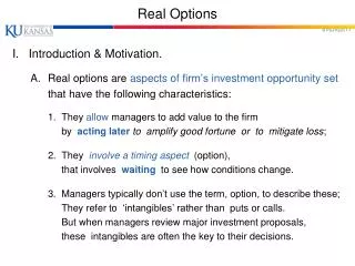
1. Real Options I. Introduction & Motivation. A. Real options are aspects of firm’s investment opportunity set that have the following characteristics: 1. They allow managers to add value to the firm by actinglater to amplify good fortune or to mitigate loss; 2. They involve a timing aspect (option), that involves waiting to see how conditions change. 3. Managers typically don’t use the term, option, to describe these; They refer to ‘intangibles’ rather than puts or calls. But when managers review major investment proposals, these intangibles are often the key to their decisions.

2. I. Introduction & Motivation B. This discussion: 1. Describes four common and important real options: The option to expanda project later if conditions are good. The option to abandona project later if conditions are bad. The option to wait (& learn about conditions) before investing. The option to vary the firm’s output or production methods. 2. Works through some simple numerical examples to demonstrate: a. How real options can be valued; b. That valuing these options can change the investment decision. c. The technique of option valuation. C. Point: Unless you understand the basics of options & their valuation, and how these affect the firm’s investment opportunity set, you are likely to make mistakes in: - Setting up an investment problem; - Considering option valuation; - Understanding the opportunities; - Making investment decisions.

3. II. The Option to Expand a Project Later A. Example 1: Investment in the Mark I microcomputer. It’s 1982. Company expects growth in PC mkt; Considers investment in developing Mark I PC. Forecasted cash flows and NPV in following table: ____________________________________________________________________________________________________________________________________ Summary of cash flows for Mark I project (Millions of $) 1982 1983 1984 1985 1986 1987 . (1) cash flow -200 +110 +159 +295 +185 0 (2) capital investmt 250 0 0 0 0 0 (3) in working cap. 0 50 100 100 -125 -125 Net cf [(1)-(2)-(3)] -450 +60 +59 +195 +310 +125 NPV at 20% = -$46.45 MM or -$46 MM . CFO says project can’t make it on financial grounds (has NPV = -$46 MM at 20% hurdle rate), but have to do project anyway, for strategic reasons – “If we don’t do it now, later will be too late, when Apple, IBM, and others are established.” You say the actual source of strategic value is a real option – If you go ahead with the Mark I, can follow up later with Mark II, if Mark I does well. If you don’t go ahead with the Mark I now, it will be too expensive to enter the market later … Mark I gives firm not only its own cash flows, but also a call option to do the Mark II later. The call let’s you invest in the Mark II later, if it looks good, or walk away if it looks bad. CFO says, then what’s the project worth?

4. II.B. Valuing the Option to Invest in Mark II 1.Must make assumptions: a. Decision to invest in Mark II must be made after 3 years (T=3; 1985). b. Mark II investment is double in scale to the Mark I (expect growth!); Investment required will be $900 MM (exercise price), and is fixed. c. Forecasted cash inflows of Mark II are also double those of Mark I; S = NPV(exp. cash flows) = $800 / (1.2)3= $463 MM in 1982 (today). d. Future value of Mark II cash flows is highly uncertain ( = .35). e. The annual riskfree rate is 10%. 2. Interpretation: The opportunity to invest in the Mark II is a three-year European call option on an asset worth $463 MM (today), with a $900 MM exercise price. i.e., if value increases > $900 MM within three years, option will be ITM.

5. II.B. Valuing the Option to Invest in Mark II 3. Valuation: Black/Scholes Call Value = S * N(d1) - PV(K) * N(d2) where S = $463 MM; PV(K) = $900 / (1.1)3 = 676; d1 = [ln ( S / PV(K) ) / (T)½ ] + (T)½ / 2 = [ln (.685) / .606] + .606 / 2 = -.3216; d2 = d1 - (T) ½ = -.3216 - .606 = -.9216; N(d1) = .3739; N(d2) = .1767; Call Value = ($463 * .3739) - ($676 * .1767) = $53.59 MM 4. Final Decision: Opportunity to invest in Mark I has projected cash flows with NPV = -$46 MM, But this opportunity also contains a call option to invest in the Mark II, that has an additional value = $54 MM. Together, investment in the Mark I plus the call on Mark II are worth +$8 MM.

6. II.C. Discussion of Option to Invest in Mark II 1. Mark II is not expected (assumed) to be moreprofitable than Mark I, just twice as big, and therefore twice as bad in terms of discounted cash flow! But there is a chance that Mark II could be extremely valuable, if mktgrows. Value could be far above $900 MM in 1985 (remember, = .35! ). Call option allows company the ability to cash in on the upside. Today, the ability - option - to cash in on the upside is worth $54 MM. 2. This valuation is only a rough approximation. (need to make assumptions!) Analysis can be expanded to account for many other complexities encountered. This example illustrates how valuable follow-on investment opportunities can be, especially when uncertainty is high and the product market is growing rapidly. 3. In addition, Mark II will also give call options on Mark III, IV, V, … These calculations don’t take value of those subsequent real options into account.

7. II.D. Real Options and the Value of Management 1. Discounted Cash Flow (DCF) implicitly assumes firms hold real assets passively. It ignores real options found in assets. Sophisticated managers can recognize, take advantage of, and value these options. In this sense, DCF does not reflect the value of management. 2. The DCF model was first developed for evaluating bonds and stocks. Investors in these assets are necessarily passive. i.e., there is nothing investors can do to improve the interest rate they are paid, or the dividends they receive (with rare exceptions). A bond or stock can be sold, but that just substitutes one passiveinvestmtfor another. 3. Options and securities that contain options are fundamentally different. Investors in options do not have to be passive. They have a right to make a decision, which they can exercise to capitalize on good fortune, or to mitigate loss. This right has value whenever there is uncertainty. However, calculating the value of this right is not a simple matter of discounting. Option pricing theory can tell us what the value is (not DCF). • The firm is an investor in real assets. Management can add value to those assets by responding to new circumstances, by taking advantage of good fortune or mitigating loss. DCF misses the value of real options because it treats the firm as a passive investor.

8. III. The Option to Abandon a Project Later A. Example 2: 1. Must choose between two technologies to produce a new product. a. Technology A uses newer technology to produce higher volumes at lower costs. However, if product doesn’t sell, technology is worthless. b. Technology B uses older technology that produces lower volumes at higher costs (e.g., uses more labor). However, if product doesn’t sell, can sell the technology. 2. Technology A looks better with DCF analysis; a. It was designed to have lower costs at planned production volume. 3. Technology B has the advantage of flexibility. ←(valuable!) a. If you are unsure about the success of the new product, may ignore Technology A’s better DCF value, and choose Technology B for its ‘intangible’ flexibility advantage.

9. III.A. Example 2: Option to Abandon 4. Valuation: Model the flexibility of Technology B as a put option. Must make assumptions: Initial capital outlays are same for Technologies A and B. Technology A pays $18.5 MM if product is hit; $8.5 MM if not. Technology B pays $18.0 MM if product is hit; $8.0 MM if not. Think of these payoffs as cash flow in first year plus NPV of all later cash flows. ** Can abandon (sell) Technology B at end of year 1, and receive $10 MM. If you are obliged to continue production, regardless of success, pick Technology A. If you are not obliged to continue, should consider the option to sell Technology B. Technology A: Success - continue production - own business worth $18.5 MM; Failure - continue production - own business worth $8.5 MM. Technology B: Success - continue production - own business worth $18.0 MM; Failure - exercise option to sell - abandon; receive $10.0 MM. Technology B offers a put option that acts like insurance; If market fails, can abandon project and recover $10 MM (> $8 MM!). This abandonment opportunity is a put option with exercise price (K) = $10 MM.

10. III.A. Example 2: Option to Abandon Note: The total value of the project using Technology B is its DCF value, assuming the company does not abandon, plusthe value of the abandonment put option. When you value this put option, you are placing value on flexibility. 5. Additional Assumptions regarding project and Technology B: a. Suppose project would be worth $12 MM today if it could not be abandoned. This is the value of the underlying asset today. b. If demand is good in one year, value increases to $18 MM. If demand is bad in one year, value decreases to $8 MM. If demand is good, company will wish to continue. If demand is bad, company can abandon & receive $10 MM. c. Suppose riskfree rate = 5% (1+r = 1.05).

11. III.A. Example 2: Option to Abandon 6. Payoffs fit the one-period binomial model (u = 1.5; d = .67). Success: project worth $18 MM; put option worth $0. Failure: project worth $8 MM; put option worth $10 - $8 = $2 MM. ● $18 (fu = $0) $12 (?) ● (p = $1.03 MM) ● $8 (fd = $2) Future values of abandonment option are in parentheses. Need to compute the NPV of expected payoffs. Probability of success: p = ((1+r)-d)/(u-d) = (1.05-.67)/(1.5-.67) = .46; Value of put = [exp. payoff] / (1+r) = [(.46)*($0) + (.54)*($2)] / 1.05 = $1.03 MM 7. Without abandonment option, project worth $12.00 MM; With abandonment option, project worth $13.03 MM.

12. IV. The Timing Option A. Optimal investment timing is easy when no uncertainty. Simply compute the NPV at various future investment dates and pick date that gives highest current value. Problem: if there is uncertainty, this simple rule breaks down. B. Suppose your project could be big winner or loser; Upside outweighs downside; has positive NPV if done today. However, project is not ‘now-or-never.’ Could wait & invest later. Problem: If project is winner, waiting means loss of early cash flows. If project is loser, waiting could prevent big losses. This Positive NPV project is an in-the-money Americancall option. Optimal investment timing means exercising at the best time.

13. IV.C. Example 3: Investment is not ‘Now-or-Never’ C. Investment Opportunity: Construct factory for $180 MM. 1. First assumeit’s a now-or-never opportunity. If NPV > 0, this is an in-the-money European call that’s about to expire. (Then it has only intrinsic value). The call’s payoff is its NPV. If NPV < 0, out-of-the-money, payoff is zero. The payoff is the intrinsic value of the call (broken line graph). 2. Next assumeyou can waita year. Now option has extrinsic value. Even though option has NPV < 0 now, option has value since you can wait to see if market takes off. value of option to invest | investment | can be postponed | | investment | now or never | |__________________________________________________ Project NPV K

14. IV.C. Example 3: Investment is not ‘Now-or-Never’ 3. Opportunity to invest now or wait is an American calloption. Tradeoff; exercising option to invest now means you no longer benefit from volatility. Option holders like volatility! It means upside potential! Furthermore, the option to wait limits possible loss. On the other hand, waiting means you forgo cash flows. If the cash flows (NPV) are high enough, will gladly exercise now! ← (like dividend) The project’s cash flows play same role as dividend payments on a stock. When a stock does not pay dividends, American call is always worth more alive. But div payment before option matures reduces the ex-div price & payoffs later. Want to exerciseAmerican options just before dividend is paid. * Dividends do not always prompt early exercise, but if they are large enough, call option holders capture them by exercising just before the ex-dividend date. * Managers act same way. When project’s forecasted cash flows are sufficiently large, managers ‘capture’ the cash flows by investing immediately. When cash flows small, managers are reluctant to commit to positive NPV projects. Caution is rational, as long as option to wait is open and valuable enough. This value depends on NPV & volatilityof forecasted cash flows.

15. IV.D. Valuation of Timing Option Assume:i. If you commit $180 MM now, have project worth NPV = $200 MM. ←(ITM $20MM) ii. If demand is low in year 1, cash flow = $16 and project worth $160. If demand is high in year 1, cash flow = $25 and project worth $250. ← iii. Investment cannot be postponed beyond 1 year. (NPV of E(CF) at year 1) If you invest now, capture first year’s cash flow ($16 MM or $25 MM); If you invest later, miss first year’s cash flow, but will have more information later. “Probability of success”: If demand is high, cash flow = $25 and year-end value = $250; Then total return = ($25 + $250) / $200 = 1.375 (+37.5%). If demand is low, cash flow = $16 and year-end value = $160; Then total return = ($16 + $160) / $200 = .88 ( -12%). Thus, p = ( (1+r) - d) / (u-d) = (1.05 -.88) / (1.375 -.88) = .34; (1-p) = .66. Want to value American call with K = $180 MM: ● $250 (fu = NPV = $250-$180 = $70) ●cash flow = 25 $200 (?) ● ● cash flow = 16 At end of year: ● $160 (fd = $0) If project value = $160, option is OTM (worth $0). If project value = $250, option is ITM ($70). Value of call = [ .34 ($70) + .66 ($0) ] / 1.05 = $22.9 MM. Invest now, project worth NPV= $20 MM; Invest later, project worth call value = $22.9 MM. Invest later ! Option worth more alive.

16. V. Flexible Production Facilities A. Consider a sheep: nota flexibleproduction facility. 1. Produces wool & mutton in roughly fixed proportions. 2. If price of wool rises and price of mutton falls, cannot respond. B. Manufacturing facilities can be flexible. 1. May vary output mix as demand changes. 2. Companies also try to avoid dependence on single source of raw mtls. C. Utilities are allotted emission allowances; specific amtof sulfur dioxide. 1. These allowances can be traded; a. Utility may choose to reduce emissions or buy more allowances. b. There are ways to reduce emissions: i. Burn expensive low-sulfur coal; ii. Invest in co-firing equipment (allows firm to switch from natural gas to coal). c. This flexibility is valuable: i. If cost of emission allowances rises, or price of natural gas falls, cofiring could prove to be a cheaper means of production. ii. Investing in co-firing equipment gives an option to switch between different means of production to meet changing costs.

17. V. Flexible Production Facilities D. Auto manufacturers. 1. Toyota has manufacturing operations in Japan, U.S., and other countries. 2. As relative costs of production change across countries, with changing labor costs and exchange rates, Toyota can switch production location to where costs are relatively cheap. E. In these examples, Firm acquires an option to exchange one risky asset for another. These are complex. Real Option analysis can be adapted to value these.

18. VI. Too Simple? A. Valuation in the above examples requires unrealistic assumptions about the distribution of prices, when using Black/Scholes, or about u & d, when using Binomial Model. 1. The numbers in these examples give an idea of what can be done. However, the numbers indicated by Black/Scholes or Binomial Model are ‘bad,’ in that they require unrealistic assumptions. 2. Further, the valuation explanations above apply to tradedoptions. What about real options? a. If options are not traded freely, can no longer use arb. arguments. Risk neutral valuation (B/S or Binomial) still makes sense. Just an application of certainty-equivalent (risk-neutral) method. The key assumption is that company’s shareholders have access to assets with the same risk characteristics (e.g., same beta) as the capital investments being evaluated by the firm.

19. VI. Too Simple? c. Think of each real investment opportunity has having a ‘double’: - traded security with identical risk. Then expected return for the double is also the cost of capital for the real investment, and the discount rate for a DCF valuation of the project. d. Now what would investors pay for real option based on project? The same as for an identical traded option written on the double! This traded option does not have to exist; It is enough to know how it would be valued by investors, who could use either the arbitrage or the risk-neutral method. The two methods give the same answer. e. When we value a real option by the risk-neutral method, we are calculating the option’s value as if it could be traded. This parallels the standard capital budgeting approach. A DCF calculation of project NPV is an estimate of the project’s market value IF the project could be set up as a mini-firm with shares traded on the stock market. The certainty-equivalent (risk-neutral) value of a real option is likewise an estimate of option’s market value IF it were traded.

20. VI. Too Simple? 3. The true value of applying Real Option analysis is in helping managers to organize the problem to be attacked. a. This framework allows managers to clearly specify what are the factors that affect the value of the project. b. Consideration of these factors is crucial to help managers make good decisions.