
Unsupervised Learning: Estimating Cluster Tree from Sample Data
E N D
Presentation Transcript
Unsupervised Learning: Estimating the Cluster Tree of a Density by Analyzing the Minimal Spanning Tree of a Sample Werner Stuetzle Professor and Chair, StatisticsAdjunct Professor, Computer Science and EngineeringUniversity of Washington, Seattle Supported by NSF grant DMS-9803226 and NSA grant 62-1942. Work performed while on sabbatical at AT&T Labs - Research.
1. Introduction • Given:Collection of n objects, characterized by feature vectors x1, … , xn. • General goal of unsupervised learning: • Detect presence of distinct groups • Assign objects to groups • Note: Important to distinguish between unsupervised learningandcompact partitioning • Unsupervised learning: Identify distinct groups • Compact partitioning:Partition collection of objects into compact strata
The prototypical compact partitioning method:K-means clustering • Let Pk = P1 ,…, Pk be a partition of the observations into k groups. • Measure badness of a partition by the sum of squared distances of observations from their group means: • Find optimal partition (for example with the Lloyd algorithm) • Note: • K-means clustering can be successful at finding groups if • we picked the correct k • groups are roughly spherical, and • approximately of the same size • For the remainder of the talk, will focus on unsupervised learning
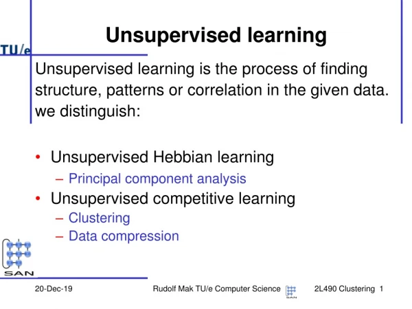
2. Approaches to Unsupervised Learning • Regard feature vectors x1, … , xn as sample from some density p(x) • Parametric approach: (Cheeseman, McLachlan, Raftery) • Based on premise that each group g is represented by density pg that is a member of some parametric family => p(x) is a mixture • Estimate the parameters of the group densities, the mixing proportions, and the number of groups from the sample. • Nonparametric approach: (Wishart, Hartigan) • Based on the premise that distinct groups manifest themselves as multiple modes of p(x) • Estimate modes from sample • Will pursue nonparametric approach
3. Describing the modal structure of a density Consider feature vectors x1 , …. , xn as a sample from some density p(x) . Define level set L(c ; p) as the subset of feature space for which the density p(x) is greater than c. Note: Level sets with multiple connected components indicate multi-modality There might not be a single level set that reveals all the modes
The cluster tree of a density • Modal structure of density is described by cluster tree. • Each node N of cluster tree • represents a subset D(N) of feature space • is associated with a density level c(N) • Root node • represents the entire feature space • is associated with density level c(N) = 0 • Tree defined recursively: to determine descendents of node N • Find lowest level c for which intersection of D(N) with L(c ; p) has two connected components • If there is no such c then N is leaf of tree; leaves of tree <==> modes • Otherwise, create daughter nodes representing the connected components, with associated level c
Goal: Estimate the cluster tree of the underlying density p(x) from the sample feature vectors x1 , …. , xn First step: Estimate p(x) by density estimate p*(x) Second step: Compute cluster tree of p*
Problem: For most density estimates, finding connected components of level sets is hard. Need to resort to heuristics. Notable exception: 1-near-neighbor density estimate. Can find level sets exactly by analyzing the minimal spanning tree of the sample.
4. The minimal spanning tree and 1-near-neighbor density estimation • Minimal spanning tree • Given: Feature vectors x1 , …. , xn and distance measure on feature space • (Euclidean)minimal spanning tree = graph connecting x1 , …. , xn with smallest total edge length. • Has been used for multivariate two-sample tests, mapping data into lower dimensions, skeletonizing point sets, ….. • Prim’s principles for MST construction: • Any point can be connected to its nearest neighbor • Any tree fragment can be connected to its nearest neighbor by the shortest possible link
One-near-neighbor density estimation • Given: X = {x1 ,…., xn} sample from unknown density p(x) • The 1-nn density estimate is defined as • p*(x) ~ 1 / dk(x, X) • where k is the dimensionality • Note: Not a very good density estimate • Cannot be normalized • Has a singularity at each data point • However, we are primarily interested in connected components of level sets, so flaws are not necessarily fatal.
Connection between MST and 1-nn density estimation T(d) : subgraph of MST obtained by removing all edges of length > d T(d) defines partition P of data set X L(c ; p*) : level set of 1-nn density estimate p*(x) for level c L(c ; p*) defines a partition Q of data set X Proposition (Hartigan 1985): For every density threshold c there is a corresponding edge length threshold d such that the resulting partitions P and Q are identical. Can find level sets of 1-nn density estimate by analyzing the MST
5. Constructing a cluster tree from the MST Problem: 1-nn density estimate is very noisy --- singularity at each observation => cluster tree would have n leaves Idea: Control size of cluster tree byrunt size thresholdSplit of connected component of L(c, p*) is considered “significant” if both daughter components are larger than runt size threshold. Sketch of algorithm Repeat { Break longest edge of MST} Until min (size of left subtree, size of right subtree) > runt size threshold If … apply recursively to subtrees
rs = 2 rs = 1 rs = 5 • Runt analysis • Define runt size (J. H.) of MST edge e: • Break all MST edges that are longer than e • runt_size (e) = min (#obs in left subtree, #obs in right subtree) Algorithm: compute_cluster_tree (mst, runt_size_threshold) { node = new_cluster_tree_node; node.leftson = node.rightson = NULL; node.obs = leaves (mst); cut_edge = longest_edge_with_large_runt_size (mst, runt_size_threshold); if (cut_edge) { node.leftson = compute_cluster_tree (left_subtree(mst, cut_edge), runt_size_threshold); node.rightson = compute_cluster_tree (right_subtree(mst, cut_edge), runt_size_threshold); } return(node); }
Heuristic justification: MST edges with large runt size indicate presence of multiple modes • Recall multi-fragment algorithm for MST construction: • Define distance d (G1, G2) between groups as minimum distance between observations • Initialize each obs to form its own group • Repeat { Find closest groups Add shortest edge connecting them Merge closest groups} Until only one group remains • What will happen? • Fragments will start and grow in high density regions, where distances are small • Eventually, those fragments will be joined by edges • Those edges will have large runt size
Illustration Left: data setMiddle: rootogram of runt sizesRight: MST after removal of all edges with length > length (edge with largest runt size)
Computational complexity • Computing MST: O (n log n) using spatial hashing • Computing runt sizes for edges of MST: O (n log n) • Deciding on whether a cluster with m observations should be split: O (m) • However • Spatial partitioning most effective if n large relative to d.
Relationship to single linkage clustering • Single linkage clustering = standard way of extracting clusters from MSTTo obtain k clusters, break k-1 longest edges in MST • Problems: • Breaking longest edges tends to separate stragglers from the bulk of the data and often results in one large and many small clusters (“chaining”) • Choosing a single threshold for edge length <=> choosing a single cut level for 1-NN density estimate. However, there might not be a single cut level that reveals all the leaves of the mode tree. Cut at upper level reveals two leftmost modes. Cut at lower level reveals right mode. Need to consider cuts at all levels
6. Illustration - olive oil data Objects: 572 olive oil samples coming from 9 different areas, grouped into 3 regions (1, 2, 3, 4) (5, 6) (7, 8, 9) Features: Concentration of 8 different chemicals Question: How well canwe recover the grouping into regions and areas Note:To evaluate performance of unsupervised learning methods, need labeled data 20 largest runt sizes: 168 97 59 51 42 42 33 13 13 12 11 11 11 10 10 8 8 8 8 7 Fairly clear gap: Choose runt size 33 as threshold Note: Situation not always that clear cut
Estimate of cluster tree, olive oil data • Interpretation: • Bottom split separates region 3 from regions 1, 2 • Next split on left separates region 1 from region 2 • Not able to correctly partition region 1 into areas
Areas vs clusters: Interpretation of table: There are 25 olive oil samples from area 1. One of them ended up in cluster 2, 17 in cluster 6, and 7 in cluster 8 Not able to recognize areas 1- 4 in region 1
Diagnostic plot: Do the two clusters in area 3 really correspond to modes ? (a) cluster tree with node splitting area 3 selected; (b) projection of data in node on Fisher discriminant direction separating daughters; (c) cluster tree with node separating area 3 from area 2 selected; (d) projection of data on Fisher direction
Diagnostic plot: Do areas 1 and 4 really correspond to modes ? Projection of areas 1 (black), 2 (green), 3 (blue), and 4 (red) on the plane spanned by first two discriminant coordinates Note: Not an operational diagnostic --- assumes knowledge of true labels
Comparative evaluation • Have run a number of experiments on simulated data and data sets from machine learning. • Competitive with other methods that make implicit assumptions about shape of groups (model based clustering, average linkage ..) • A lot better when assumptions made by those methods are violated.
7. Summary and future work • The term “clustering” is ambiguous --- need to distinguish between compact partitioning and unsupervised learning. • Goal of unsupervised learning: detect presence of distinct groups. • Assumption: groups ~ modes --- connected components of level sets --- of feature density. • This definition accommodates elongated and non-linear groups. • Modal structure of density is described by cluster tree. • Cluster tree is defined recursively --- suggests recursive partitioning. • Potentially many variations on basic algorithm, differing in • (1) estimate of feature density (2) heuristic for deciding when to split a node • Attractive choice: 1-near-neighbor density estimate. Level sets and their connected components can be found exactly by analyzing minimal spanning tree of sample
Future work • Principled method for deciding on number of groups --- hard! • Sampling or aggregation methods for dealing with large data sets • Visualization: Link cluster tree with other displays such as histograms, scatterplots, etc, to understand location and shape of clusters in feature space • Quantitative evaluation and comparison of methods • Thank you for your attention