Value at Risk By A.V. Vedpuriswar
580 likes | 928 Vues
Value at Risk By A.V. Vedpuriswar. October 31 , 2010. Introduction. Value at Risk (VAR) is probably the most important tool for measuring market risk. VAR tells us the maximum loss a portfolio may suffer at a given confidence interval for a specified time horizon.

Value at Risk By A.V. Vedpuriswar
E N D
Presentation Transcript
Value at RiskBy A.V. Vedpuriswar October 31, 2010
Introduction • Value at Risk (VAR) is probably the most important tool for measuring market risk. • VAR tells us the maximum loss a portfolio may suffer at a given confidence interval for a specified time horizon. • If we can be 95% sure that the portfolio will not suffer more than $ 10 million in a day, we say the 95% VAR is $ 10 million.
Illustration • Average revenue = $5.1 million per day • Total no. of observations = 254. • Std dev = $9.2 million • Confidence level = 95% • No. of observations < - $10 million = 11 • No. of observations < - $ 9 million = 15 • Find 95% VAR. 5
Find the point such that the no. of observations to the left = (254) (.05) = 12.7 (12.7 – 11) /( 15 – 11 ) = 1.7 / 4 ≈ .4 So required point = - (10 - .4) = - $9.6 million VAR = E (W) – (-9.6) = 5.1 – (-9.6) = $14.7 million If we assume a normal distribution, Z at 95% ( one tailed) confidence interval = 1.645 VAR = (1.645) (9.2) = $ 15.2 million
Problem • The VAR on a portfolio using a one day horizon is USD 100 million. What is the VAR using a 10 day horizon ? • Solution • Variance scales in proportion to time. • So variance gets multiplied by 10 • And std deviation by √10 • VAR = 100 √10 = (100) (3.16) = 316 • (σN2 = σ12 + σ22 ….. = Nσ2) • Note; This approach is valid only when the daily variances are independent. 7
Problem • If the daily VAR is $12,500, calculate the weekly, monthly, semi annual and annual VAR. Assume 250 days and 50 weeks per year. • Solution • Weekly VAR = (12,500) (√5) = 27,951 • Monthly VAR = ( 12,500) (√20) = 55,902 • Semi annual VAR = (12,500) (√125) = 139,754 • Annual VAR = (12,500) (√250) = 197,642 8
We have a portfolio of $10 million in shares of Microsoft. We want to calculate VAR at 99% confidence interval over a 10 day horizon. The volatility of Microsoft is 2% per day. Calculate VAR. Problem • Solution • σ = 2% = (.02) (10,000,000) = $200,000 • Z (P = .01) = Z (P =.99) = 2.33 • Daily VAR = (2.33) (200,000) = $ 466,000 • 10 day VAR = 466,000 √10 = $ 1,473,621 10 Ref : John C Hull, Options, Futures and Other Derivatives
Problem • Consider a portfolio of $5 million in AT&T shares with a daily volatility of 1%. Calculate the 99% VAR for 10 day horizon. • Solution • σ = 1% = (.01) (5,000,000) = $ 50,000 • Daily VAR = (2.33) (50,000) = $ 116,500 • 10 day VAR = $ 111,6500 √10 = $ 368,405 Ref : John C Hull, Options, Futures and Other Derivatives 11
Problem • Now consider a combined portfolio of AT&T and Microsoft shares. Assume the returns on the two shares have a bivariate normal distribution with the correlation of 0.3. What is the portfolio VAR.? • Solution • σ2 = w12σ12 + w22 σ22 + 2 ῤPw1 W2σ1σ2 • = (200,000)2 + (50,000)2 + (2) (.3) (200,000) (50,000) • σ = 220,277 • Daily VAR = (2.33) (220,277) = 513,129 • 10 day VAR = (513,129) √10 = $1,622,657 • Effect of diversification = (1,473,621 + 368,406) – (1,622,657) = 219,369 12 Ref : John C Hull, Options, Futures and Other Derivatives
Problem • Consider a portfolio with two foreign currencies, Canadian dollar and euro. These two currencies are uncorrelated and have a volatility against the dollar of 5% and 12% respectively. The portfolio has $2 million invested in CAD and $1 million in Euro. What is the portfolio VAR at 95% confidence level? • Variance of the portfolio return • = {(2 (.05)}2 + {(1) (.12)}2 =.01 + .0144 = .0244 • Std devn = √.0244 = $ .156205 million • VAR = (1.65) (156,205) = $257,738 • VAR for Canadian dollar part = $ (1.65) (.05) (2) million = $165,000 • VAR for Euro part = $ (1.65) (.12) (1) million = $ 198,000 • Undiversified VAR = $ 363,000 • Thus the diversified VAR is significantly lower.
Problem • Suppose we increase the Canadian dollar position by $10,000. What is the marginal VAR? • Variance = {(2.01) (.05)}2 + {(1) (.12)}2=.0101 + .0144= .0245 • σ= √.0245 = $.1565 million • VAR = (1.65) (156,500) = $ 258,225 • Marginal VAR = 258,225 – 257,738 = $ 487
Problem • Consider a position consisting a $100,000 investment in asset A and a $100,000 investment in asset B. Assume that the daily volatilities of both assets are 1% and that the coefficient of correlation between their returns is 0.3. What is the 5-day 99% VaR for the portfolio? • Solution • The standard deviation of the daily change in the investment in each asset is $1,000. The variance of the portfolio’s daily change is • 1,0002 + 1,0002 + 2 x 0.3 x 1,000 x 1,000 = 2,600,000 • The standard deviation of the portfolio’s daily change is $1,612.45. • The standard deviation of the 5-day change is • 1,612.45 x √5 = $3,605.55 • From the tables of N(x) we see that N (-2.33) = 0.01. • The 5-day 99 percent value at risk is therefore 2.33 x 3,605.55 = $8,401. Ref : John C Hull, Options, Futures and Other Derivatives
Problem • A financial institution owns a portfolio of options on the US dollar-sterling exchange rate. The delta of the portfolio is 56.0. The current exchange rate is $/£ 1.5000. Derive an approximate linear relationship between the change in the portfolio value and the percentage change in the exchange rate. If the daily volatility of the exchange rate is 0.7%, estimate the 10-day 99% VaR. • Solution • The approximate relationship between the daily change in the portfolio value, ΔP, and the daily change in the exchange rate, ΔS, is ΔP = 56 ΔS • For a unit change in £, $ will change by 1.5. It follows that • ΔP = 56 x 1.5 Δx • Or ΔP = 84 Δx • The standard deviation of Δx equals the daily volatility of the exchange rate, or 0.7 percent.The standard deviation of ΔP is therefore 84 x 0.007 = $ 0.588. • So the 10-day 99 percent VaR for the portfolio is • 0.588 x 2.33 x √10 = $ 4.33 for an investment of £1. Ref : John C Hull, Options, Futures and Other Derivatives
Problem • Some time age a company entered into a forward contract to buy £1 million for $1.5 million. The contract now has 6 months to maturity. The daily volatility of a 6-month zero-coupon sterling bond (when its price is translated to dollars) is 0.06% and the daily volatility of a 6-month zero-coupon dollar bond is 0.05%. The correlation between returns from the two bonds is 0.8. The current exchange rate is $/ £ 1.53. Calculate the standard deviation of the change in the dollar value of the forward contract in 1 day. What is the 10-day 99% VaR? Assume that the 6-month interest rate in both sterling and dollar is 5% per annum with continuous compounding. • The contract is a long position in a sterling bond plus a short position in a dollar bond. • The value of the sterling bond is 1.53e-0.05x0.5 or $1.492 million. • The value of the dollar bond is 1.5e-0.05x0.5 or $1.463 million. • The variance of the change in the value of the contract in one day is : • 1.4922 x 0.00062 + 1.4632 x 0.00052 – 2 x 0.8 x 1.492 x 0.0006 x 1.463 x 0.0005 = 0.000000288 • The standard deviation is therefore $0.000537 million. • The 10-day 99% VaR is $0.000537 x √10 x 2.33 = $0.00396 million Ref : John C Hull, Options, Futures and Other Derivatives
Problem Consider the contract on the dollar/euro exchange rate (EC) traded on the CME. The notional amount is 125,000 Euros. Assume that the annual volatility is 12% and the current price is $1.05 per Euro. Find daily VAR at 99% confidence level. Solution VAR = (2.33) [(.12) / √252] × (125,000 × 1.05) = $ 2310 18
Problem • Consider a portfolio with a one day VAR of $1 million. Assume that the market is trending with an auto correlation of 0.1. Under this scenario, what would you expect the two day VAR to be? • Solution • V2 = 2σ2 (1 + ῤ) • = 2 (1)2 (1 + .1) = 2.2 • V = √2.2 = 1.4832
Auto correlation over longer periods Consider a period of 5 days. We assume the first day’s movement will have an impact on the second day's movement through the correlation coefficient. The first day’s movement will affect the third day’s movement through the square of the correlation coefficient and so on. Then the combined variance will be: σ2 + σ2 + σ2 + σ2 + σ2 + (2) () σ2 + (2) ()2σ2 + (2) ()3σ2 + (2) ()4σ2 + (2) () σ2 + (2) ()2 σ2 + (2) ()3 σ2 + (2) () σ2 + (2) ()2σ2+ (2) () σ2 = 5 σ2 + (8) () σ2 + (6) ()2σ2 + (4) ()3σ2 + (2) ()4σ2
σ = .1 ; = .3 • Variance = (5) (.1)2 + (4) (2) (.3) (.1)2 • + (3) (2) (.3)2 (.1)2 + (2) (2) (.3)3 (.1)2 • + (2) (.3)4 (.1)2 • = .05 + .024 + .0054 + .00108 + .000162 • = .080642 • Volatility = .284 Consider a portfolio with standard deviation of daily returns of 0.1 and autocorrelation of 0.3. Calculate the 5 day volatility.
What is Monte Carlo VAR? • The Monte Carlo approach involves generating many price scenarios (usually thousands) to value the assets in a portfolio over a range of possible market conditions. • The portfolio is then revalued using all of these price scenarios. • Finally, the portfolio revaluations are ranked to select the required level of confidence for the VAR calculation.
Step 1: Generate Scenarios • The first step is to generate all the price and rate scenarios necessary for valuing the assets in the relevant portfolio, as well as the required correlations between these assets. • There are a number of factors that need to be considered when generating the expected prices/rates of the assets: • Opportunity cost of capital • Stochastic element • Probability distribution
Opportunity Cost of Capital • A rational investor will seek a return at least equivalent to the risk-free rate of interest. • Therefore, asset prices generated by a Monte Carlo simulation must incorporate the opportunity cost of capital.
Stochastic Element • A stochastic process is one that evolves randomly over time. • Stock market and exchange rate fluctuations are examples of stochastic processes. • The randomness of share prices is related to their volatility. • The greater the volatility, the more we would expect a share price to deviate from its mean.
Probability Distribution • Monte Carlo simulations are based on random draws from a variable with the required probability distribution, usually the normal distribution. • The normal distribution is useful when modeling market risk in many cases. • But it is the returns on asset prices that are normally distributed, not the asset prices themselves. • So we must be careful while specifying the distribution.
Step 2: Calculate the Value of the Portfolio • Once we have all the relevant market price/rate scenarios, the next step is to calculate the portfolio value for each scenario. • For an options portfolio, depending on the size of the portfolio, it may be more efficient to use the delta approximation rather than a full option pricing model (such as Black-Scholes) for ease of calculation. • Δoption = Δ(ΔS) • Thus the change in the value of an option is the product of the delta of the option and the change in the price of the underlying.
Other approximations • There are also other approximations that use delta, gamma (Γ) and theta (Θ) in valuing the portfolio. • By using summary statistics, such as delta and gamma, the computational difficulties associated with a full valuation can be reduced. • Approximations should be periodically tested against a full revaluation for the purpose of validation. • When deciding between full or partial valuation, there is a trade-off between the computational time and cost versus the accuracy of the result. • The Black-Scholes valuation is the most precise, but tends to be slower and more costly than the approximating methods.
Step 3: Reorder the Results • After generating a large enough number of scenarios and calculating the portfolio value for each scenario: • the results are reordered by the magnitude of the change in the value of the portfolio (Δportfolio) for each scenario • the relevant VAR is then selected from the reordered list according to the required confidence level • If 10,000 iterations are run and the VAR at the 95% confidence level is needed, then we would expect the actual loss to exceed the VAR in 5% of cases (500). • So the 501st worst value on the reordered list is the required VAR. • Similarly, if 1,000 iterations are run, then the VAR at the 95% confidence level is the 51st highest loss on the reordered list.
Formula used typically in Monte Carlo for stock price modelling
Advantages of Monte Carlo • We can cope with t risks associated with non-linear positions. • We can choose data sets individually for each variable. • This method is flexible enough to allow for missing data periods to be excluded from the VAR calculation. • We can incorporate factors for which there is no actual historical experience. • We can estimate volatilities and correlations using different statistical techniques.
Problems with Monte Carlo • Cost of computing resources can be quite high. • Speed can be slow. • RandomNumbers may not be all that random. • Pseudo random numbers are only a substitute for true random numbers and tend to show clustering effects. • Monte Carlo often assumes normal distribution. • But it can be performed with alternative distributions. • Results (value at risk estimate) depend critically on the models used to value (often complex) financial instruments.
Introduction • Unlike the Monte Carlo approach, it uses the actual historical distribution of returns to simulate the VAR of a portfolio. • Real data plus ease of implementation, have made historical simulation a very popular approach to estimating VAR. • Historical simulation avoids the assumption that returns on the assets in a portfolio are normally distributed. • Instead, it uses actual historical returns on the portfolio assets to construct a distribution of potential future portfolio losses. • This approach requires minimal analytics. • All we need is a sample of the historic returns on the portfolio whose VAR we wish to calculate.
Steps • Collect data • Generate scenarios • Calculate portfolio returns • Arrange in order.
What is VAR (90%) ? 10% of the observations, i.e, (.10) (30) = 3 lie below -7 So VAR = -7
Advantages and Disadvantages of Historical simulation • Advantages • Simple • No normality assumption • Non parametric • Disadvantages • Reliance on the past • Length of estimation period • Weighting of data
Simulation vs Variance Covariance • Simulation approaches are preferred by global banks due to: • flexibility in dealing with the ever-increasing range of complex instruments in financial markets • the advent of more efficient computational techniques in recent years • the falling costs in information technology • However, the variance-covariance approach might be the most appropriate method for many smaller firms, particularly when: • they do not have significant options positions • they prefer to outsource the data requirement component of their risk calculations to a company such as RiskMetrics • significant savings can often be made by using outsourced volatility and correlation data, compared to internally storing the daily price histories required for simulation techniques
Basel Committee Standards • Banks that prefer to use internal models must meet, on a daily basis, a capital requirement that is the higher of either: • the previous day's value at risk • the average of the daily value at risk of the preceding 60 business days multiplied by a minimum factor of three • VAR must be computed on a daily basis. • A one-tailed confidence interval of 99% must be used. • The minimum holding period should be 10 trading days . • The minimum historical observation period should be one year.
Banks should update their data sets at least once every three months. • Banks can recognize correlations within broad risk categories. • Provided the relevant supervisory authority is satisfied with the bank's system for measuring correlations , they may also recognize correlations across broad risk factor categories. • Banks' internal models are required to accurately capture the unique risks associated with options and option-like instruments. • The Basel Committee has also specified qualitative factors that banks must meet before they are permitted to use internal models.
The Basel Committee prescribes an increase in capital requirements if, based on a sample of 250 observations (a one-year observation period), the VAR model underpredicts the number of exceptions (losses exceeding the 99% confidence level). • For such purposes, three 'zones' have been distinguished by the Committee. • Green Zone : 0-4 exceptions • Yellow zone : 5-9 exceptions • Red zone : 10 or more exceptions
Problem • Based on a 90% confidence level, how many exceptions in back testing a VAR should be expected over a 250 day trading year? • 10% of the time loss may exceed VAR • So no. of observations = (.10) (250) • = 25 45
Problem We are currently feeding a model with 600 days of data. The VAR confidence level is 99%. One exception is observed. Should we reject the model? Solution Probability of no exception = (.99)600 = .0024 Probability of one exception = 600 (.99)599 (.01) = .0146 Total probability = .017 < .05 So we reject the model at 5% confidence level. Ref : John C Hull, Options, Futures and Other Derivatives
Problem We back test a VAR model with 1000 days of data. The VAR confidence level is 99%. 17 exceptions are observed. Should the model be rejected at 5% confidence level? Solution The probability of the VAR being exceeded on a given day = 1 - .99 = .01 The probability of the VAR being exceeded on 17 days or more =1 – Binomdist (16, 1000, .01, True) = 2.64% 2.64% < 5% So the model should be rejected. Ref : John C Hull, Options, Futures and Other Derivatives
Introduction • Stress testing involves analysing the effects of exceptional events in the market on a portfolio's value. • These events may be exceptional, but they are also plausible. • And their impact can be severe. • Historical scenarios or hypothetical scenarios can be used.