Download
1 / 35
350 likes | 487 Vues
Mobile Ad hoc Networks COE 549 Routing Protocols I. Tarek Sheltami KFUPM CCSE COE www.ccse.kfupm.edu.sa/~tarek. Outline. Routing Algorithms Classifications Proactive Routing: Table Driven Protocols Cluster-based Protocols. Routing Algorithm Classifications. Routing Algorithms.

E N D
Mobile Ad hoc Networks COE 549Routing Protocols I Tarek Sheltami KFUPM CCSE COE www.ccse.kfupm.edu.sa/~tarek
Outline • Routing Algorithms Classifications • Proactive Routing: • Table Driven Protocols • Cluster-based Protocols
Routing Algorithm Classifications Routing Algorithms Proactive Reactive Hybrid • Table Driven • Cluster-based • On-Demand • Cluster-based
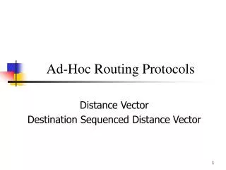
Table Driven Protocols • Distance Vector Protocols such as: • Wireless Routing Protocol (WRP) [MUR96] • Destination Sequenced Distance Vector (DSDV) routing protocol [PER94] • Least Resistance Routing (LRR) [PUR93] • The protocol by Lin and Liu [LIN99]. • Link State Protocols such as: • Global State Routing (GSR) [CHE98] • Fisheye State Routing (FSR) [PEI00a] • Adaptive Link-State Protocol (ALP) [PEI00a] • Source Tree Adaptive Routing (STAR) [ACE99] • Optimized Link State Routing (OLSR) protocol [SHE03b] • Landmark Ad Hoc Routing (LANMAR) [PEI00b] • However the most prominent protocol is DSDV
Table Driven Protocols • Try to match the link state and distance vector ideas to the wireless environment • Each node only needs to know the next hop to the destination, and how many hops away the destination is: • This information stored in each node is often arranged in a table, hence the term “table-driven routing” • Such algorithm are often called distance vector algorithms, because nodes exchange vectors of their known distances to all other nodes • An example is the Bellman-Ford algorithm, one of the first ones to be used for routing in the Internet
Bellman-Ford Algorithm • Consider a collection of nodes, connected over bi-directional wired links of given delays. • We want to find the fastest route from each node to any other node. • An example network: • Initially, each node knows the distances to its direct neighbors, and stores them to its routing table. Nodes other than their direct neighbors are assumed to be at an infinite distance. • Then, nodes start exchanging their routing tables.
Table Driven Protocols • As the number of nodes n increases, the routing overhead increases very fast, like O(n2). • When the topology changes, routing loops may form:
Destination Sequenced Distance Vector (DSDV) • One of the earlier ad hoc routing protocols developed • Its advantage over traditional distance vector protocols is that it guarantees loop freedom • Extends the classical DBF by tagging each distance entry dik(j) by a sequence number (SN) that is originated by the destination node j. • Each routing table, at each node, contains a list of the addresses of every other node in the network • Along with each node’s address, the table contains the address of the next hop for a packet to take in order to reach the node • In addition to the destination address and next hop address, routing tables maintain the route metric and the route sequence number.
Destination Sequenced Distance Vector (DSDV).. • The update packet starts out with a metric of one • The neighbors will increment this metric and then retransmit the update packet. • This process repeats itself until every node in the network has received a copy of the update packet with a corresponding metric • If a node receives duplicate update packets, the node will only pay attention to the update packet with the smallest metric and ignore the rest
Destination Sequenced Distance Vector (DSDV).. • To distinguish stale update packets from valid ones, the original node tags each update packet with a sequence number • The sequence number is a monotonically increasing number, which uniquely identifies each update packet from a given node • If a node receives an update packet from another node, the sequence number must be equal to or greater than the sequence number already in the routing table; otherwise the update packet is stale and ignored • If the sequence number matches the sequence number in the routing table, then the metric is compared and updated as previously discussed
Disadvantages of DSDV Protocol • Routing is achieved by using routing tables maintained by each node • The bulk of the complexity in generating and maintaining these routing tables • If the topological changes are very frequent, incremental updates will grow in size • This overhead is DSDV’s main weakness, as Broch et al. [BRO98] found in their simulations of 50-node networks
Virtual Base Station (VBS) • All nodes are eligible to become clusterhead / VBS • Each node is at one hop from its clusterhead • Clusterhead / VBS is selected based on the smallest ID • Gateways / Boarder Mobile Terminals (BMTs) • Clsuterheads and Gatewaysform the virtual backbone of the network
VBS.. • Every MT has an ID number, sequence number and my_VBS variable • Every MT increases its sequence number after every change in its situation • An MT my_VBS variable is set to the ID number of its VBS; however, if that MT is itself a VBS, then the my_VBS variable will be set to 0, otherwise it will be set to –1, indicating that it is a VBS of itself
CGSR infrastructure Creation • CGSR uses the Least Cluster Change (LCC) clustering algorithm • No clusterheads in the same transmission range • Each Cluster has a different code to eliminate the interference, typically the suggest 4 Walsh codes
Range of node #1 Some issues about pure Cluster-based Routing (VBS) Routing in VBS
Some issues about pure Cluster-based Routing (VBS) Routing in VBS
Drawback of VBS • All the nodes require the aid of their VBS(s) all the time, so this results a very high MAC contention on the VBSs • the periodic hello message updates are not efficiently utilized by MTs (other than VBSs and BMTs) • The power of the nodes with small IDs drain down much faster than that with large IDs