Download
1 / 44
440 likes | 555 Vues
Understand the key factors affecting stock option prices, risk-return tradeoffs, profit profiles, and bounds on market prices through comprehensive analysis of options trading strategies.

E N D
ASSUMPTIONS: 1. The market is frictionless: No transaction cost nor taxes exist. Trading are executed instantly. There exists no restrictions to short selling.2. Market prices are synchronous across assets. If a strategy requires the purchase or sale of several assets in different markets, the prices in these markets are simultaneous. Moreover, no bid-ask spread exist; only one trading price.
3. Risk-free borrowing and lending exists at the unique risk-free rate. Risk-free borrowing is done by sellingT-bills short and risk-free lending is done by purchasing T-bills. 4. There exist no arbitrage opportunities in the options market
NOTATIONS: t = the current date. St= the market price of the underlying asset. K = the option’s exercise (strike) price. T = the option’s expiration date. T-t = the time remaining to expiration. r = the annual risk-free rate. • = the annual standard deviation of the returns on the underlying asset. D = cash dividend per share. q = The annual dividend payout ratio.
FACTORS AFFECTING OPTIONS PRICES: Ct = the market premium of an American call. ct = the market premium of an European call. Pt = the market premium of an American put. pt = the market premium of an European put. In general, we express the premiums as functions of the following variables: Ct , ct= c{St , K, T-t, r, , D }, Pt , pt= p{St , K, T-t, r, , D }.
Options Risk-Return Tradeoffs PROFIT PROFILE OF A STRATEGY A graph of the profit/loss as a function of all possible market values of the underlying asset We will begin with profit profiles at the option’s expiration; I.e., an instant before the option expires.
Options Risk-Return Tradeoffs At Expiration 1. Only at expiry; T. 2. No time value; T-t = 0 CALL is: exercised if ST > K expires worthless if ST K Cash Flow = Max{0, ST – K} PUT is: exercised if ST < K expires worthless if ST≥K Cash Flow = Max{0, K – ST}
3. All parts of the strategy remain open till expiry. 4. A Table Format Every row is one part of the strategy. Every row is analyzed independently of the other rows. The total strategy is the vertical sum of the rows. The profit is the cash flow at expiration plus the initial cash flows of the strategy, disregarding the time value of money.
5. A Graph of the profit/loss profile The profit/loss from the strategy as a function of all possible prices of the underlying asset at expiration.
The algebraic expressions of P/L at expiration: Long stock: –St + ST Short stock: St - ST Long call: -ct + Max{0, ST - K} Short call: ct + Min{0, K - ST} Long put: -pt + Max{0, K - ST} Short put: pt + Min{0, ST - K} Notice: the time value of money is ignored.
Borrowing and Lending: In many strategies with lending or borrowing capital at the risk-free rate, the amount borrowed or lent is the discounted value of the option’s exercise price: Ke-r(T-t). The strategy’s holder can buy T-bills (lend) or sell short T-bills (borrow) for this amount. At the option’s expiration, the lender receives K. If borrowed, the borrower will pay K, namely, a cash flow of – K.
Bounds on options market prices Call values at expiration: CT = cT = Max{ 0, ST – K }. Proof: At expiration the call is either exercised, in which case CF = ST – K, or it is left to expire worthless, in which case, CF = 0.
Minimum call value: A call premium cannot be negative. At any time t, prior to expiration, Ct , ct 0. Proof: The current market price of a call is the NPV[Max{ 0, ST – K }] 0.
(Sec.9.3 p.209) Maximum Call value:Ct St. Proof: The call is a right to buy the stock. Investors will not pay for this right more than the value that the right to buy gives them, I.e., the stock itself.
Put values at expiration: PT = pT = Max{ 0, K - ST}. Proof: At expiration the put is either exercised, in which case CF = K - ST, or it is left to expire worthless, in which case CF = 0.
Minimum put value: A put premium cannot be negative. At any time t, prior to expiration, Pt , pt 0. Proof: The current market price of a put is The NPV[Max{ 0, K - ST}] 0.
(Top p.210) Maximum American Put value: At any time t < T, Pt K. Proof: The put is a right to sell the stock For K, thus, the put’s price cannot exceed the maximum value it will create: K, which occurs if S drops to zero.
Maximum European Put value: Pt Ke-r(T-t). Proof: The maximum gain from a European put is K, ( in case S drops to zero). Thus, at any time point before expiration, the European put cannot exceed the NPV{K}.
Lower bound: American call value: At any time t, prior to expiration, Ct Max{ 0, St - K}. Proof: Assume to the contrary that Ct < Max{ 0, St - K}. Then, buy the call and immediately exercise it for an arbitrage profit of: St – K – Ct > 0; a contradiction of the no arbitrage profits assumption.
Eq(9.1)p.211Lower bound: European call value: At any t, t < T, ct Max{ 0, St - Ke-r(T-t)}. Proof: If, to the contrary, ct < Max{ 0, St - Ke-r(T-t)}, then, 0 < St - Ke-r(T-t) - ct At expiration StrategyI.C.FST < KST > K Sell stock short St -ST -ST Buy call - ct 0 ST - K Lend funds - Ke-r(T-t) K K Total ? K – ST 0
The market value of an American call is at least as high as the market value of a European call. Ct ct Max{ 0, St - Ke-r(T-t)}. Proof: An American call may be exercised at any time, t, prior to expiration, t<T, while the European call holder may exercise it only at expiration.
Lower bound: American put value: At any time t, prior to expiration, Pt Max{ 0, K - St}. Proof: Assume to the contrary that Pt < Max{ 0, K - St}. Then, buy the put and immediately exercise it for an arbitrage profit of: K - St – Pt > 0. A contradiction of the no arbitrage profits assumption.
Sec. 9.6An American put is always priced higher than an European put. Pt pt Max{0, Ke-r(T-t) - St}. Proof: An American put may be exercised at any time, t, prior to expiration, t < T, while a European put may be exercise at expiration. If the price of the underlying asset fall below some price, it becomes optimal to exercise the American put. At that very same moment the European put holder wants to (optimally) exercise the put but cannot because it is a European put.
The put-call parity. European options: The premiums of European calls and puts written on the same non dividend paying stock for the same expiration and the same strike price must satisfy: ct - pt = St - Ke-r(T-t). The parity may be rewritten as: ct + Ke-r(T-t) = St + pt. Proof:
At expiration Strategy I.C.FST < KST > K Buy stock -StSTST Buy put - pt K - ST 0 Total -(St+pt) K ST At expiration Strategy I.C.FST < KST > K Buy call - ct0ST-K Lend - Ke-r(T-t) K K Total -(ct+ Ke-r(T-t) ) K ST
Synthetic European options: The put-call parity ct + Ke-r(T-t = St + pt can be rewritten as a synthetic call: ct = pt + St - Ke-r(T-t), or as a synthetic put: pt = ct - St + Ke-r(T-t).
The put-call parity for American options (Eq.(9.4) p.215) The premiums on American options satisfy the following inequalities: St - K < Ct - Pt < St - Ke-r(T-t).
Proof: Rewrite the inequality: St - K < Ct - Pt < St - Ke-r(T-t). The RHS of the inequality follows from the parity for European options: ct - pt = St - Ke-r(T-t). The stock does not pay dividend, thus, Ct = ct. For the American puts, however, Pt > pt. Next, suppose that: St - K > Ct - Pt or, St - K - Ct + Pt > 0. This is an arbitrage profit making strategy, which contradicts the supposition above.
Early exercise: Non dividend paying stock It is not optimal to exercise an American call prior to its expiration if the underlying stock does not pay any dividend during the life of the option. Proof: If an American call holder wishes to rid of the option at any time prior to its expiration, the market premium is greater than the intrinsic value because the time value is always positive.
The American feature is worthless if the underlying stock does not pay out any dividend during the life of the call. Mathematically: Ct = ct. Proof: Follows from the previous result.
It can be optimal to exercise an American put on a non dividend paying stock early. Proof: There is still time to expiration and the stock price fell to 0. An American put holder will definitely exercise the put. It follows that early exercise of an American put may be optimal if the put is enough in-the money.
For S< S** the European put premium is less than the put’s intrinsic value. For S< S* the American put premium coincides with the put’s intrinsic value. P/L American put is always priced higher than its European counterpart. Pt pt K Ke-r(T-t) P p S* S** K S
Early exercise: The dividend effect Early exercise of Unprotected American calls on a cash dividend paying stock: Consider an American call on a cash dividend paying stock. It may be optimal to exercise this American call an instant before the stock goes x-dividend. Two condition must hold for the early exercise to be optimal: First, the call must be in-the-money. Second, the $[dividend/share], D, must exceed the time value of the call at the X-dividend instant. To see this result consider:
FACTS: 1. The share price drops by $D/share when the stock goes x-dividend. 2. The call value decreases when the price per share falls. 3. The exchanges do not compensate call holders for the loss of value that ensues the price drop on the x-dividend date. SCUMD SXDIV tPAYMENT tAnnouncement tXDIV Time line 4. SXDIV = SCDIV - D.
The call holder goal is to maximize the Cash flow from the call. Thus, at any moment in time, exercising the call is inferior to selling the call. This conclusion may change, however, an instant before the stock goes x-dividend: ExerciseDo not exercise Cash flow: SCD – K c{SXD, K, T - tXD} Substitute: SCD = SXD + D. Cash flow: SXD –K + D SXD – K + TV.
Conclusion: Early exercise of American calls may be optimal: 1. The call must be in the money And 2. D > TV. In this case, the call should be (optimally) exercised an instant before the stock goes x-dividend and the cash flow will be: SXD –K + D.
Early exercise of Unprotected American calls on a cash dividend paying stock: The previous result means that an investor is indifferent to exercising the call an instant before the stock goes x dividend if the x- dividend stock price S*XD satisfies: S*XD –K + D = c{S*XD , K, T - tXD}. It can be shown that this implies that the Price, S*XD ,exists if: D > K[1 – e-r(T – t)].
Eq.(9.7) p.219 The put-call parity. European options: Suppose that European puts and calls are written on a dividend paying stock. There will be n dividend Payments in the amounts Dj on dates tj; j = 1,…,n, tn < T. rj = the risk-free rate during tj – t; j=1,…,n,T. Then,
j = 1,…,n At expiration Strategy I.C.FtjST < KST > K Sell stock St -Dj - ST - ST sell put ptST - K 0 Buy call - ct0ST- K Lend - Ke-rT(T-t) K K Lend - Dje-rj(tj-t) Dj Total 0 0 0 0
Eq(9.8) p.219 When the options are written on a dividend paying stock the RHS of the inequality remains the same : Ct - Pt < St - Ke-r(T-t). Assuming two dividend payments, the LHS of the inequality becomes: St - K – D1e-r(t1-t) – D2 e-r(t2-t) < Ct - Pt
A Risk-free rate with options: A Box spread: K1 < K2 At expiration StrategyICFST< K1K1<ST < K2 ST > K2 Buy p(K2) -p2 K2- ST K2– ST 0 Sell p(K1) p1 ST - K1 0 0 Sell c(K2) c20 0 K2 - ST Buy c(K1) -c1 0 ST - K1 ST - K1 Total ? K2-K1 K2-K1 K2-K1 Therefore, the initial investment is riskless. c1 - c2 + p2 - p1 = (K2-K1)e-r(T-t)
RESULTS for PUTS and CALLS: 33. Box spread: Again: An initial investment of c1 - c2 + p2 - p1 yields a sure cash flow of K2-K1. Thus, arbitrage profit exists if the rate of return on this investment is not equal to the T-bill rate which matures on the date of the options’ expiration. c1 - c2 + p2 - p1 = (K2-K1)e-r(T-t)