Download
1 / 42
420 likes | 647 Vues
Yan Y. Kagan Dept. Earth and Space Sciences, UCLA, Los Angeles, CA 90095-1567, ykagan@ucla.edu, http://scec.ess.ucla.edu/ykagan.html. GLOBAL EARTHQUAKE PREDICTION EXPERIMENTS. http://moho.ess.ucla.edu/~kagan/csep06.ppt. Earthquake Occurrence – Stochastic Process.

E N D
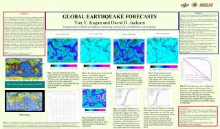
Yan Y. Kagan Dept. Earth and Space Sciences, UCLA, Los Angeles, CA 90095-1567, ykagan@ucla.edu, http://scec.ess.ucla.edu/ykagan.html GLOBAL EARTHQUAKE PREDICTION EXPERIMENTS http://moho.ess.ucla.edu/~kagan/csep06.ppt
Earthquake Occurrence – Stochastic Process • Multidimensional marked (seismic moment, M) (or tensor-valued) point process in time, space, and 3-D orientation of double-couple focal mechanism -T x R3 x SO(3). • All the marginal distributions are power-law, i.e., they are fractal, heavy-tailed, stable (L-stable) distributions.
NEW STATISTICS – STABLE DISTRIBUTIONS Statistics development over last two centuries has been dominated by the Gaussian distribution – a special case of stable laws. Other stable distributions have completely different properties: mean, standard deviation, coefficient of correlation either does not exist or behaves erratically. The stable distributions theory started to be developed only 20 years ago and there are not enough statisticians who sufficiently know it. Zaliapin, Kagan, Schoenberg, PAGEOPH, 162, 2005.
DIFFERENTIAL GEOMETRY, GROUP THEORY • Earthquake focal mechanisms sometimes undergo large random 3-D rotations. To describe a set of focal mechanisms we need to have a statistical theory of 3-D rotations. The group SO(3) is non-commutative (the sum of two rotations depends on its order), its theory is very complicated. We need to involve mathematicians to develop methods appropriate to handling random rotations and random tensors. See more in http://scec.ess.ucla.edu/~ykagan/india_index.html
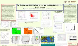
Earthquake size distribution Tapered Gutenberg-Richter distribution of scalar seismic moment, survival function Moment threshold Exponent, similar to b-value Corner moment
Review of results on spectral slope, b: Although there are variations, none is significant with 95%-confidence. Kagan’s [1999] hypothesis of uniform b still stands.
. Moment rate vs. tectonic rate By integrating the distribution of seismic moment we obtain relation between seismic moment rate, seismic activity rate, beta, and corner moment: Kagan, GJI, 149, 731-754, 2002; Bird and Kagan, BSSA, 94(6), 2380-2399, 2004; Boettcher & Jordan, JGR, 109(B12), B12302, 2004.
Relation between moment sums and tectonic deformation Now that we know the coupled thickness of seismogenic lithosphere in each tectonic setting, we can convert surface velocity gradients to seismic moment rates. Now that we know the frequency/magnitude distribution in each tectonic setting, we can convert seismic moment rates to earthquake rate densities at any desired magnitude. Long-term-average (Poissonian) seismicity maps Kinematic Model Moment Rates
De Mare, J., Optimal prediction of catastrophes with applications to Gaussian processes, Ann. Probability, 8, 841-850, 1980. Molchan, G. M., and Y. Y. Kagan, 1992. Earthquake prediction and its optimization, J. Geophys. Res., 97, 4823-4838.
Earthquake Probability Forecasting • The fractal dimension of earthquake process is lower than the embedding dimension: • Time – 0.5 in 1D • Space – 2.2 in 3D • Focal mechanisms – Cauchy distribution • This allows us to forecast probability of earthquake occurrence – specify regions of high probability, use temporal clustering for evaluating possibility of new event and predict its focal mechanism.
(a) Earthquake catalog data Phenomenological models: (b) Point process branching along magnitude axis, introduced by Kagan (1973a;b) (c) Point process branching along time axis (Hawkes, 1971; Kagan & Knopoff, 1987; Ogata, 1988)
Long-term forecast: 1977-today Spatial smoothing kernel is optimized by using the first, temporal, part of a catalog to forecast its second part.
Time history of long-term and hybrid (short-term plus 0.8 * long-term) forecast for a point at latitude 39.47 N., 143.54 E. northwest of Honshu Island, Japan. Blue line is the long-term forecast; red line is the hybrid forecast.
Short-term forecast uses Omori's law to extrapolate present seismicity. Red spot north of Kamchatka is a recent (2006/4/20) M7.6 earthquake
Kagan, Y. Y., D. D. Jackson, and Y. F. Rong, 2006. A testable five-year forecast of moderate and large earthquakes in southern California based on smoothed seismicity, Seism. Res. Lett., submitted.
Helmstetter, A., Y. Y. Kagan, and D. D. Jackson, 2006. Comparison of short-term and time-independent earthquake forecast models for southern California, Bull. Seismol. Soc. Amer., 96(1), 90-106.
Here we demonstrate forecast effectiveness: displayed earthquakes occurred after smoothed seismicity forecast was calculated.
Forecast Efficiency Evaluation • We simulate synthetic catalogs using smoothed seismicity map. • Likelihood function for simulated catalogs and for real earthquakes in the time period of forecast is computed. • If the `real earthquakes’ likelihood value is within 2.5—97.5% of synthetic distribution, the forecast is considered successful. Kagan, Y. Y., and D. D. Jackson, 2000. Probabilistic forecasting of earthquakes, (Leon Knopoff's Festschrift), Geophys. J. Int., 143, 438-453.
Molchan, G. M., and Y. Y. Kagan, 1992. Earthquake prediction and its optimization, J. Geophys. Res., 97, 4823-4838.
Kossobokov, 2006. Testing earthquake prediction methods: ``The West Pacific short-term forecast of earthquakes with magnitude MwHRV \ge 5.8", Tectonophysics, 413(1-2), 25-31. See also Kagan & Jackson, Tectonophysics, pp.33-38.
. Likelihood ratio – information/eq We approximate earthquake occurrence by Poisson cluster process and calculate the earthquake rate Likelihood function is
. Likelihood ratio – information/eq Similarly we obtain likelihood function for the null hypothesismodel (Poisson process in time) Information content of a catalog : (bits/earthquake) characterizes uncertainty reduction by use of a particular model. Kagan and Knopoff, PEPI, 1977; Kagan, GJI, 1991; Kagan and Jackson, GJI, 2000; Helmstetter, Kagan and Jackson, BSSA, 2006
. Likelihood ratio – information/eq • Because of power-law dependence of earthquake rate on time (Omori’s law), the likelihood function (l) approaches infinity when the prediction horizon is close to zero (i.e., for real-time earthquake prediction). • Similarly, when spatial resolution of earthquake data increases, (l) again goes to infinity. • Molchan diagram also approaches the ideal state for the prediction horizon close to zero, or if the location accuracy significantly increases.
Kagan, Y. Y., and H. Houston, 2005. Relation between mainshock rupture process and Omori's law for aftershock moment release rate, Geophys. J. Int., 163(3), 1039-1048
Branching Model for Dislocations (Kagan and Knopoff, JGR,1981; Kagan, GJRAS, 1982) • Predates use of self-exciting, ETAS models which also have branching structure. • A more complex model, exists on a more fundamental level. • Continuum-state critical branching random walk in T x R3 x SO(3).
Simulated source-time functions and seismograms for shallow earthquake sources. The upper trace is a synthetic source-time function. The middle plot is a theoretical seismogram, and the lower trace is a convolution of the derivative of source-time function with the theoretical seismogram. Kagan, Y. Y., and Knopoff, L., 1981. Stochastic synthesis of earthquake catalogs, J. Geophys. Res., 86, 2853-2862.
Snapshots of fault propagation (intersection with a plane). Rotation of focal mechanisms is modeled by the Cauchy distribution. Integers in the frames # indicate the numbers of elementary events to which these frames correspond. Frames show the development of an earthquake sequence.
Kagan, Y. Y., and Knopoff, L., 1984. A stochastic model of earthquake occurrence, Proc. 8-th Int. Conf. Earthq. Eng., 1, 295-302.
Conclusions • Using universality of the distribution of earthquake size (seismic moment) we quantitatively describe plate tectonic deformation end evaluate long-term earthquake rate. • Time-independent seismic hazard is evaluated by optimized smoothing of past seismicity.
Conclusions • Temporal earthquake occurrence is modeled and forecasted by a multidimensional branching process. • Finally, kinematic continuum-state critical branching process can be used to generate whole earthquake rupture process and obtain a randomized set of seismograms – extrapolation of the process.
Probabilistic vs. alarm forecasts A modern scientific earthquake forecast should be quantitatively probabilistic. In 1654 Pierre de Fermat and Blaise Pascal exchanged letters in which they founded the quantitative probability theory. Now more than 350 years later, any earthquake forecast without direct use of probability has a medieval flavor. This is perhaps the reason the general public and media are so attracted to yes/no forecasts. No probability – no prediction