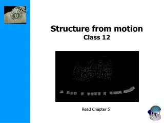
Structure from motion Class 9
Structure from motion Class 9. Read Chapter 5. TexPoint fonts used in EMF. Read the TexPoint manual before you delete this box.: A A A A A A. Geometric Computer Vision course schedule (tentative). Today’s class. Structure from motion factorization sequential bundle adjustment.

Structure from motion Class 9
E N D
Presentation Transcript
Structure from motionClass 9 Read Chapter 5 TexPoint fonts used in EMF. Read the TexPoint manual before you delete this box.: AAAAAA
Today’s class • Structure from motion • factorization • sequential • bundle adjustment
Factorization • Factorise observations in structure of the scene and motion/calibration of the camera • Use all points in all images at the same time • Affine factorisation • Projective factorisation
Affine camera The affine projection equations are how to find the origin? or for that matter a 3D reference point? affine projection preserves center of gravity
All equations can be collected for all i and j • where Orthographic factorization (Tomasi Kanade’92) The ortographic projection equations are where Note that P and M are resp. 2mx3 and 3xn matrices and therefore the rank of m is at most 3
Orthographic factorization (Tomasi Kanade’92) Factorize m through singular value decomposition An affine reconstruction is obtained as follows Closest rank-3 approximation yields MLE!
Orthographic factorization (Tomasi Kanade’92) Factorize m through singular value decomposition An affine reconstruction is obtained as follows • A metric reconstruction is obtained as follows • Where A is computed from 3 linear equations per view on symmetric matrix C (6DOF) A can be obtained from C through Cholesky factorisation and inversion
Examples Tomasi Kanade’92, Poelman & Kanade’94
Examples Tomasi Kanade’92, Poelman & Kanade’94
Examples Tomasi Kanade’92, Poelman & Kanade’94
Examples Tomasi Kanade’92, Poelman & Kanade’94
Perspective factorization The camera equations for a fixed image i can be written in matrix form as where
Perspective factorization All equations can be collected for all i as where In these formulas m are known, but Li,P and M are unknown Observe that PM is a product of a 3mx4 matrix and a 4xn matrix, i.e. it is a rank-4 matrix
Perspective factorization algorithm Assume that Li are known, then PM is known. Use the singular value decomposition PM=US VT In the noise-free case S=diag(s1,s2,s3,s4,0, … ,0) and a reconstruction can be obtained by setting: P=the first four columns of US. M=the first four rows of V.
Iterative perspective factorization When Li are unknown the following algorithm can be used: 1. Set lij=1 (affine approximation). 2. Factorize PMand obtain an estimate of P andM. If s5 is sufficiently small then STOP. 3. Use m, P and M to estimate Li from the cameraequations (linearly) miLi=PiM 4. Goto 2. In general the algorithm minimizes the proximity measure P(L,P,M)=s5 Note that structure and motion recovered up to an arbitrary projective transformation
Further Factorization work Factorization with uncertainty Factorization for dynamic scenes (Irani & Anandan, IJCV’02) (Costeira and Kanade ‘94) (Bregler et al. ‘00, Brand ‘01) (Yan and Pollefeys, ‘05/’06)
practical structure and motion recovery from images • Obtain reliable matches using matching or tracking and 2/3-view relations • Compute initial structure and motion • Refine structure and motion • Auto-calibrate • Refine metric structure and motion
Initialize Motion (P1,P2 compatibel with F) Sequential Structure and Motion Computation Initialize Structure (minimize reprojection error) Extend motion (compute pose through matches seen in 2 or more previous views) Extend structure (Initialize new structure, refine existing structure)
Computation of initial structure and motion according to Hartley and Zisserman “this area is still to some extend a black-art” • All features not visible in all images • No direct method (factorization not applicable) • Build partial reconstructions and assemble (more views is more stable, but less corresp.) 1) Sequential structure and motion recovery 2) Hierarchical structure and motion recovery
Sequential structure and motion recovery • Initialize structure and motion from two views • For each additional view • Determine pose • Refine and extend structure • Determine correspondences robustly by jointly estimating matches and epipolar geometry
Initial structure and motion Epipolar geometry Projective calibration compatible with F Yields correct projective camera setup (Faugeras´92,Hartley´92) Obtain structure through triangulation Use reprojection error for minimization Avoid measurements in projective space
Determine pose towards existing structure M 2D-3D 2D-3D mi+1 mi new view 2D-2D Compute Pi+1using robust approach (6-point RANSAC) Extend and refine reconstruction
Compute P with 6-point RANSAC • Generate hypothesis using 6 points • Count inliers • Projection error • 3D error • Back-projection error • Re-projection error • Projection error with covariance • Expensive testing? Abort early if not promising • Verify at random, abort if e.g. P(wrong)>0.95 (Chum and Matas, BMVC’02)
Calibrated structure from motion • Equations more complicated, but less degeneracies • For calibrated cameras: • 5-point relative motion (5DOF) Nister CVPR03 • 3-point pose estimation (6DOF) Haralick et al. IJCV94 D. Nistér, An efficient solution to the five-point relative pose problem, In Proc. IEEE Computer Society Conference on Computer Vision and Pattern Recognition (CVPR 2003), Volume 2, pages. 195-202, 2003. R. Haralick, C. Lee, K. Ottenberg, M. Nolle. Review and Analysis of Solutions of the Three Point Perspective Pose Estimation Problem. Int’l Journal of Computer Vision, 13, 3, 331-356, 1994.
5-point relative motion (Nister, CVPR03) • Linear equations for 5 points • Linear solution space • Non-linear constraints scale does not matter, choose 10 cubic polynomials
5-point relative motion (Nister, CVPR03) represents polynomial of degree n in z • Perform Gauss-Jordan elimination on polynomials -z -z -z
Three points perspective pose – p3p (Haralick et al., IJCV94) All techniques yield 4th order polynomial Haralick et al. recommends using Finsterwalder’s technique as it yields the best results numerically 1841 1903
Minimal solvers Lot’s of recent activity using Groebner bases: • Henrik Stewénius, David Nistér, Fredrik Kahl, Frederik Schaffalitzky: A Minimal Solution for Relative Pose with Unknown Focal Length,CVPR 2005. • H. Stewénius, D. Nistér, M. Oskarsson, and K. Åström. Solutions to minimal generalized relative pose problems. Omnivis 2005. • D. Nistér, A Minimal solution to the generalised 3-point pose problem, CVPR 2004 • Martin Bujnak, Zuzana Kukelova, Tomás Pajdla: A general solution to the P4P problem for camera with unknown focal length. CVPR 2008. • Brian Clipp, Christopher Zach, Jan-Michael Frahm and Marc Pollefeys, A New Minimal Solution to the Relative Pose of a Calibrated Stereo Camera with Small Field of View Overlap, ICCV 2009. • Zuzana Kukelova, Martin Bujnak, Tomás Pajdla: Automatic Generator of Minimal Problem Solvers. ECCV 2008. • …
Changchang’sSfM code • for iconic graph • uses 5-point+RANSAC for 2-view initialization • uses 3-point+RANSAC for adding views • performs bundle adjustment • For additional images • use 3-point+RANSAC pose estimation
Hierarchical structure and motion recovery • Compute 2-view • Compute 3-view • Stitch 3-view reconstructions • Merge and refine reconstruction F T H PM
Stitching 3-view reconstructions Different possibilities 1. Align (P2,P3) with (P’1,P’2) 2. Align X,X’ (and C’C’) 3. Minimize reproj. error 4. MLE (merge)
Refining structure and motion • Minimize reprojection error • Maximum Likelyhood Estimation (if error zero-mean Gaussian noise) • Huge problem but can be solved efficiently (Bundle adjustment)
Non-linear least-squares • Newton iteration • Levenberg-Marquardt • Sparse Levenberg-Marquardt
Newton iteration Jacobian Taylor approximation normal eq.
Levenberg-Marquardt Normal equations Augmented normal equations accept solve again l small ~ Newton (quadratic convergence) l large ~ descent (guaranteed decrease)
Levenberg-Marquardt Requirements for minimization • Function to compute f • Start value P0 • Optionally, function to compute J (but numerical ok, too)
Sparse Levenberg-Marquardt • complexity for solving • prohibitive for large problems (100 views 10,000 points ~30,000 unknowns) • Partition parameters • partition A • partition B (only dependent on A and itself)
Sparse bundle adjustment residuals: normal equations: with note: tie points should be in partition A
Sparse bundle adjustment normal equations: modified normal equations: solve in two parts:
P1 P2 P3 M U1 U2 W U3 WT V 3xn (in general much larger) 12xm Sparse bundle adjustment Jacobian of has sparse block structure im.pts. view 1 Needed for non-linear minimization
U-WV-1WT WT V 3xn 11xm Sparse bundle adjustment • Eliminate dependence of camera/motion parameters on structure parameters Note in general 3n >> 11m Allows much more efficient computations e.g. 100 views,10000 points, solve 1000x1000, not 30000x30000 Often still band diagonal use sparse linear algebra algorithms
Sparse bundle adjustment normal equations: modified normal equations: solve in two parts:
Sparse bundle adjustment • Covariance estimation
Related problems • On-line structure from motion and SLaM (Simultaneous Localization and Mapping) • Kalman filter (linear) • Particle filters (non-linear)
Open challenges • Large scale structure from motion • Complete building • Complete city