Neuro-Fuzzy Control
Neuro-Fuzzy Control. Adriano Joaquim de Oliveira Cruz NCE/UFRJ adriano@nce.ufrj.br. Neuro-Fuzzy Systems. Usual neural networks that simulate fuzzy systems Introducing fuzziness into neurons. ANFIS architecture. Adaptive Neuro Fuzzy Inference System

Neuro-Fuzzy Control
E N D
Presentation Transcript
Neuro-Fuzzy Control Adriano Joaquim de Oliveira Cruz NCE/UFRJ adriano@nce.ufrj.br
Neuro-Fuzzy Systems • Usual neural networks that simulate fuzzy systems • Introducing fuzziness into neurons
ANFIS architecture • Adaptive Neuro Fuzzy Inference System • Neural system that implements a Sugeno Fuzzy model.
Sugeno Fuzzy Model • A typical fuzzy rule in a Sugeno fuzzy model has the form If x is A and y is B then z = f(x,y) • A and B are fuzzy sets in the antecedent. • z=f(x,y)is a crisp function in the consequent. • Usually z is a polynomial in the input variables x and y. • When z is a first-order polynomial the system is called a first-order Sugeno fuzzy model.
Sugeno Fuzzy Model z1=p1x+q1y+r1 m m A1 B1 w1 y x m m B2 A2 w2 y x z2=p2x+q2y+r2
Sugeno First Order Example • If x is small then y = 0.1x + 6.4 • If x is median then y = -0.5x + 4 • If x is large then y = x – 2 Reference: J.-S. R. Jang, C.-T. Sun and E. Mizutani, Neuro-Fuzzy and Soft Computing
Sugeno Second Order Example • If x is small and y is small then z = -x + y +1 • If x is small and y is large then z = -y + 3 • If x is large and y is small then z = -x + 3 • If x is large and y is large then z = x + y + 2 Reference: J.-S. R. Jang, C.-T. Sun and E. Mizutani, Neuro-Fuzzy and Soft Computing
Layer 1 Layer 2 Layer 3 Layer 4 Layer 5 x y A1 w1 x O1,2 P N A2 f S B1 P N y w2 B2 x y ANFIS Architecture • Output of the ith node in the l layer is denoted as Ol,i
ANFIS Layer 1 • Layer 1: Node function is • x and y are inputs. • Ai and Bi are labels (e.g. small, large). • m(x) can be any parameterised membership function. • These nodes are adaptive and the parameters are called premise parameters.
ANFIS Layer 2 • Every node output in this layer is defined as: • T is T-norm operator. • In general, any T-norm that perform fuzzy AND can be used, for instance minimum and product. • These are fixed nodes.
ANFIS Layer 3 • The ith node calculates the ratio of the ith rule’s firing strength to the sum of all rules’ firing strength • Outputs of this layer are called normalized firing strengths. • These are fixed nodes.
ANFIS Layer 4 • Every ith node in this layer is an adaptive node with the function • Outputs of this layer are called normalized firing strengths. • pi, qi and ri are the parameter set of this node and they are called consequent parameters.
ANFIS Layer 5 • The single node in this layer calculates the overall output as a summation of all incoming signals.
ANFIS Layer 5 • Every ith node in this layer is an adaptive node with the function • Outputs of this layer are called normalized firing strengths.
Alternative Structures • The structure is not unique. • For instance layers 3 and 4 can be combined or weight normalisation can be performed at the last layer.
S / Alternative Structure cont. Layer 1 Layer 2 Layer 3 Layer 4 Layer 5 x y A1 w1 S x P A2 f O1,2 B1 P y w2 B2 x y
Training Algorithm • The function f can be written as • There is a hybrid learning algorithm based on the least-squares method and gradient descent.
Example • Modeling the function • Input range [-10,+10]x[-10,+10] • 121 training data pairs • 16 rules, with four membership functions assigned to each input. • Fitting parameters = 72; 24 premise and 48 consequent parameters.