Fuzzy PID Control
Fuzzy PID Control. Jan Jantzen jj@inference.dk www.inference.dk 2013. Summary. Reduce design choices Tuning. Design Procedure. Build and tune a conventional PID controller first . Replace it with an equivalent linear fuzzy controller .

Fuzzy PID Control
E N D
Presentation Transcript
Fuzzy PID Control Jan Jantzen jj@inference.dk www.inference.dk 2013
Summary • Reduce design choices • Tuning
Design Procedure • Build and tune a conventional PID controllerfirst. • Replace it with an equivalent linear fuzzycontroller. • Make the fuzzycontroller nonlinear. • Fine-tune the fuzzycontroller. Relevant whenever PID control is possible, or already implemented
Single Loop Control Load Noise The controller should preferably be able to follow the reference r, reject load changes l and noise disturbances n, but these requirements are in conflict with each other. We would like to transfer PID tuning methods to the fuzzy controller in order to have a tuning method.
Rule Base With 4 Rules 1. If error is Neg and change in error is Neg then control is NB 3. If error is Neg and change in error is Pos then control is Zero 7. If error is Pos and change in error is Neg then control is Zero 9. If error is Pos and change in error is Pos then control is PB The four rules can handle many cases, and they are sufficient for a linear controller.
Textbook PID Controllers Continuous version Discrete version Incremental, discrete version
e E u U GE GU f Rule base Fuzzy P controller Gain on error Gain on control Provided that the rule base acts like the identity function By comparison with the P controller equation
FP Rule Base 1. If E(n) is Pos then u(n) is 100 2. If E(n) is Neg then u(n) is -100 With a proper choice of membership functions the controller will act like a linear P controller
e E GE u U f GU CE de/dt GCE Rule base Fuzzy PD Controller Provided that the rule base acts like a summation Now we know what the gains do
FPD Rule Base 1. If E(n) is Neg and CE(n) is Neg then u(n) is -200 3. If E(n) is Neg and CE(n) is Pos then u(n) is 0 7. If E(n) is Pos and CE(n) is Neg then u(n) is 0 9. If E(n) is Pos and CE(n) is Pos then u(n) is 200 With a proper choice of membership functions the controller will act like a linear PD controller. Four rules are sufficient.
e E GE u U f + GU de/dt CE + GCE PD rules IE GIE Fuzzy PD+I Controller It is better that the integral action bypasses the rule base. It saves rules.
e E GE CU cu f 1/s U GCU de/dt CE GCE Rule base Fuzzy Incremental Controller The output is a change to the previous state This is an integrator. It could be a valve position, for instance. The increment. It is a change to the sum of all previous signals.
Fuzzy - PID Gain Relation It tells what each fuzzy gain does to the proportional gain, the derivative gain, and the integral gain. Conversely, given values for Kp, Ti and Td we can find one or more sets of values for the fuzzy gains. Very important table.
Tuning Process gain If we increase Kp too much, the system might oscillate or even become unstable If we increase Kp, we suppress load changes. If we increase Kp, the response will be more sensitive to noise.
Ziegler-Nichols Tuning • Increase Kp until oscillation, Kp = Ku • Read period Tu at this setting • Use Z-N table for approximate controller gains
Ziegler-Nichols (freq. method) Given values for Ku and Tu, the table provides the gains in the three controller cases. Easy, but often the result is a poorly damped system.
Z-N oscillation of 1/(1+s)3 The ultimate gain Ku = 8, and the ultimate period is Tu = 15/4 s
PID control of 1/(1+s)3 Response to a reference step Response to a load step
Fuzzy FPD+I control of 1/(1+s)3 The response is the same as for PID control Trajectory on the control surface, which is a plane The membership functions are linear
Hand-Tuning • Set Td = 1/Ti = 0 • Tune Kp to satisfactory response, ignore any final value offset • Increase Kp, adjust Td to dampen overshoot • Adjust 1/Ti to remove final value offset • Repeat from step 3 until Kp large as possible
e E α GE u U f 1/α GU CE de/dt α GCE Rule base Scaling The linear controller is invariant towards scaling. In the nonlinear controller we can use it to avoid saturation in the input universes.
Summary • Design crisp PID • Replace it with linear fuzzy • Make it nonlinear • Fine-tune it
Kp = 4.8, Ti = 15/8, Td = 15/32 2 1 0 -1 -2 -2 0 2 Nyquist 1/(s+1)3 with PID
000 001 010 011 2 2 2 2 0 0 0 0 -2 -2 -2 -2 -2 0 2 -2 0 2 -2 0 2 -2 0 2 a) c) d) b) 101 100 110 111 2 2 2 2 0 0 0 0 -2 -2 -2 -2 -2 0 2 -2 0 2 -2 0 2 -2 0 2 e) g) h) f) Tuning Map 1/(s+1)3