Nonlinear Fuzzy PID Control
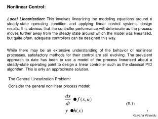
Nonlinear Fuzzy PID Control. Jan Jantzen jj@inference.dk www.inference.dk 2013. Example : a nonlinear valve. Valve opening between 0 and 1. Nonlinear flow through valve.

Nonlinear Fuzzy PID Control
E N D
Presentation Transcript
Nonlinear Fuzzy PID Control Jan Jantzen jj@inference.dk www.inference.dk 2013
Example: a nonlinear valve Valve opening between 0 and 1 Nonlinear flow through valve Three steps up on the reference. The response gets worse and worse. The third response is marginally stable and the valve saturates in the upper limit (fully open).
Standard nonlinearities Nonlinear systems can be mathematically unpredictable. Instead we simulate the behaviour using a number of standard blocks that model nonlinear components. The simulation will be approximate when we cannot solve the equations, but it is often good enough.
Standard rule base • If error is Neg and change in error is Neg then control is NB • If error is Neg and change in error is Zero then control is NM • If error is Neg and change in error is Pos then control is Zero • If error is Zero and change in error is Neg then control is NM • If error is Zero and change in error is Zero then control is Zero • If error is Zero and change in error is Pos then control is PM • If error is Pos and change in error is Neg then control is Zero • If error is Pos and change in error is Zero then control is PM • If error is Pos and change in error is Pos then control is PB With two inputs and three fuzzy terms (Neg, Zero, Pos) for each, we can build nine rules that cover the whole state space. However, just four rules may be sufficient in many cases: rules 1, 3, 7, and 9. These avoid rules with Zero, and in that case Neg and Pos must overlap each other in order to account for mid-range values.
Phase plot We have chosen one point in each quadrant Phase plane 2 1 3 Phase plot 4 Step response Trajectory of the response on the control surface Phase plane
Linear and saturationsurface We have constructed four standard control surfaces. The choice of shapes was inspired by the standard nonlinearities presented earlier. We can thus study a variety of standard behaviours. A plane. The values are between -200 and 200. The surfaces are built from four rules using these membership functions. The 'saturation' surface. The four corners are in the same positions as the linear surface.
Dead zone and quantizersurface There is a dead zone in the middle with almost zero control signal. The quantizer surface requires three input sets and nine rules. The 'quantizer' surface. The four corners are in the same positions in all four standard surfaces.
Saturation and limit cycle These are two typical phenomena in nonlinear systems. An example of saturation in the limit of the universe. The trajectory touches the edge. An example of a limit cycle. The trajectory cycles round and round for ever.
Example: unstable frictionless vehicle Force Linear equation of motion: Newton's 2. law. Acceleration Mass Design a crisp PD controller Replace it with a linear fuzzy controller Make it nonlinear (Fine-tune it)
Linear FPD Same performance as the PD controller. The PD controller was hand-tuned.
Saturation surface FPD The saturation surface provides tighter control around the centre of the surface. The response is more damped.
FPD with squared memberships Making the surface steeper improves damping even more. In this case, at least. A very good response. They are the previous ones squared. The control signal looks highly nonlinear now.
Example: nonlinear valvecompensator If u is Low then x = 4.62u If u is High then x = 0.46u + 0.543 Three steps up on the reference. The response is considerably better than without the compensator.
Example: motor actuatorwith limits Motor Actuator The control signal saturates, and the integrator in PI winds up. The response is poor.
Example: motor actuatorwith limits The response is considerably better with the FInc controller. It has an integrator at the end of its signal path, and it is relatively easy to limit it to the same limits as the actuator. It avoids windup.
Autopilot example: mass load A train car is standing on a curved track. At t = 10 the car is loaded with 5 times its own mass. It is taken off again at t = 30. A PI controller attempts to keep the train car in place (we do not consider using the brakes for the sake of the example).
Autopilot example: mass load The FInc response has a smaller dip, a smaller flare, and it avoids creeping. The PID response has a large dip, and it creeps in towards the setpoint (x = 5). This membership function is squared using Very in the rule base.
Summary • The linear fuzzy performs as a PID. • We introduced three nonlinear surfaces in order to standardize. • Fuzzy can cope with some nonlinearities that PID cannot. • Human beings can read the rule base.