Download
1 / 93
1.47k likes | 3.26k Vues
Particle size distribution. A particle population which consists of spheres or equivalent spheres with uniform dimensions is monosized and its characteristics can be described by a single diameter or equivalent diameter.

E N D
Particle size distribution • A particle population which consists of spheres or equivalent spheres with uniform dimensions is monosized and its characteristics can be described by a single diameter or equivalent diameter. • it is unusual for particles to be completely monosized, most powders contain particles with a large number of different equivalent diameters.
to be able to define a size distribution or compare the characteristics of two or more powders consisting of particles with many different diameters, the size distribution can be broken down into different size ranges, which can be presented in the form of a histogram
a histogram presents an interpretation of the particle size distribution and enables the percentage of particles having a given equivalent diameter to be determined. • A histogram representation allows different particle size distributions to be compared;
for example, the size distribution shown in Fig. (b) contains a larger proportion of fine particles than the powder in (a) in which the particles are normally distributed. • The peak frequency value, known as the mode, separates the normal curve into two identical halves, because the size distribution is fully symmetrical.
A frequency curve with an elongated tail towards higher size ranges is positively skewed (Fig. (b)); the reverse case exhibits negative skewness. • These skewed distributions can sometimes be normalized by replotting the equivalent particle diameters using a logarithmic scale, and are thus usually referred to as log normal distributions.
In some size distributions more than one mode occurs: Figure (c) shows bimodal frequency distribution for a powder which has been subjected to milling. • Some of the coarser particles from the unmilled population remain unbroken and produce a mode towards the highest particle size, whereas the fractured particles have a new mode which appears lower down the size range.
Frequency distribution curves corresponding to (a) a normal distribution, (b) a positively skewed distribution and (c) a bimodal distribution.
An alternative to the histogram representation of a particle size distribution is obtained by sequentially adding the percent frequency values as shown in Table 10.2 to produce a cumulative percent frequency distribution. • If the addition sequence begins with the coarsest particles, the values obtained will be cumulative percent frequency oversize; the reverse case produces a cumulative percent undersize.
The median particle diameter corresponds to the point that separates the cumulative frequency curve into two equal halves, above and below which 50% of the particles lie (point a in Fig. 10.5(a)). • the lower and upper quartile points at 25% and 75% divide the upper and lower ranges of a symmetrical curve into equal parts (points b and c, respectively, in Fig. 10.5(a)).
it is possible to compare two or more particle populations using the cumulative distribution representation. • For example, the size distribution in Fig. (a) shows that this powder has a larger range or spread of equivalent diameters than the powder represented in Figure (b).
Cumulative frequency distribution curves • Point a corresponds to the median • diameter. • b is the lower quartile point. • c is the upper quartile point.
Statistics • to quantify the degree of skewness of a particle population: • the interquartile coefficient of skewness (IQCS):
Where: • a is the median diameter • b is the lower quartile point • c is upper quartile point • The IQCS can take any value between -1 and +1. • If the IQCS is zero then the size distribution is practically symmetrical between the quartile points.
To quantify the degree of symmetry of a particle size distribution a property known as kurtosis can be determined. • The symmetry of a distribution is based on a comparison of the height or thickness of the tails and the 'sharpness' of the peaks with those of a normal distribution.
'Thick'-tailed 'sharp‘ peaked curves are described as leptokurtic • 'thin'-tailed 'blunt' peaked curves are platykurtic • the normal distribution is mesokurtic.
The coefficient of kurtosis, k: • where • x is any particle diameter • x is mean particle diameter • n is number of particles.
The coefficient of kurtosis has: • a value of 0 for a normal curve. • a negative value for curves showing platykurtosis. • positive values for leptokurtic size distributions.
The mean of the particle population, the median and the mode are all measures of central tendency and provide a single value near the middle of the size distribution, which represents a central particle diameter. • It is also possible to define and determine the mean in several ways and, for log-normal distributions, a series of relationships known as Hatch- Choate equations link the different mean diameters of a size distribution.
Influence of particle shape • The techniques for representing particle size distribution are all based on the assumption that particles could be adequately represented by an equivalent circle or sphere. • In some cases particles deviate markedly from circularity and sphericity. • For example, a powder consisting of monosized fibrous particles would appear to have a wider size distribution according to statistical diameter measurements.
Thus, • the breadth of the fibre could be obtained using a projected circle inscribed within the fibre di • the fibre length could be measured using a projected circle circumscribed around the fibre dc • The ratio of inscribed circle to circumscribed circle diameters can also be used as a simple shape factor to provide information about the circularity of a particle.
The ratio di /dcwill be 1 for a circle and diminish as the particle becomes more acicular.
PARTICLE SIZE ANALYSIS METHODS • Particle-size analysis methods can be divided into different categories based on several different criteria: • size range of analysis; • wet or dry methods; • manual or automatic methods; • speed of analysis.
Sieve methods • Microscope methods • Electrical stream sensing zone method (Coulter counter) • Laser light scattering methods • Sedimentation methods
Sieve methods • Equivalent diameter: • Sieve diameter, ds (the particle dimension that passes through a square aperture (length = x)).
Range of analysis • In practice sieves can be obtained for size analysis over a range from 5 to 125 000 µm.
Principle of measurement: • Sieve analysis utilizes a woven, punched or electroformed mesh, often in brass or stainless steel, with known aperture diameters which form a physical barrier to particles. • Most sieve analyses utilize a series, stack or 'nest' of sieves, which has the smallest mesh above a collector tray followed by meshes that become progressively coarser towards the top of the series.
A sieve stack usually comprises 6-8 sieves with an aperture progression based on a √2 or 2√2 change in diameter between adjacent sieves. • Powder is loaded on to the coarsest sieve of the assembled stack and the nest is subjected to mechanical vibration.
After a suitable time the particles are considered to be retained on the sieve mesh with an aperture corresponding to the sieve diameter. • Sieving times should not be arbitrary and it is recommended that sieving be continued until less than 0.2% of material passes a given sieve aperture in any 5-minute interval.
Alternative techniques: • Another form of sieve analysis, called air-jet sieving, • uses individual sieves rather than a complete nest of sieves. • Starting with the finest-aperture sieve and progressively removing the undersize particle fraction by sequentially increasing the apertures of each sieve.
Particles are encouraged to pass through each aperture under the influence of a partial vacuum applied below the sieve mesh. • A reverse air jet circulates beneath the sieve mesh, blowing oversize particles away from the mesh to prevent blocking. • Air-jet sieving is often more efficient and reproducible than using mechanically vibrated sieve analysis, although with finer particles agglomeration can become a problem.
Automatic methods: • Sieve analysis is still largely a non-automated process, although an automated wet sieving technique has been described.
Microscope methods (microscopy) • Equivalent diameters: • Projected area diameter, da • projected perimeter diameter dp • Feret's diameter dF • Martin's diameter dM
Sample preparation and analysis conditions: • Specimens prepared for light microscopy must be adequately dispersed on a microscope slide to avoidanalysis of agglomerated particles • Specimens for scanning electron microscopy are prepared by fixing to aluminium stubs before sputter coating with a film of gold a few nm in thickness. • Specimens for transmission electron microscopy are often set in resin, sectioned by microtome and supported on a metal grid before metallic coating.
Principle of measurement: • Size analysis by light microscopy is carried out on the two-dimensional images of particles oriented in three dimensions. • for dendrites, fibres or flakes it is very improbable that the particles will orient with their minimum dimensions in the plane of measurement.
Under such conditions, size analysis is carried out accepting that they are viewed in their most stable orientation. • This will lead to an overestimation of size, as the largest dimensions of the particle will be observed.
The two-dimensional images are analysed according to the desired equivalent diameter. • Using a conventional light microscope, particle-size analysis can be carried out using a projection screen with screen distances related to particle dimensions by a previously derived calibration factor using a graticule.
A graticule can also be used which has a series of opaque and transparent circles of different diameters, usually in a √2 progression. • Particles are compared with the two sets of circles and are sized according to the circle that corresponds most closely to the equivalent particle diameter being measured. • The field of view is divided into segments to facilitate measurement of different numbers of particles.
Alternative techniques: • scanning electron microscopy (SEM). • transmission electron microscopy (TEM).
Scanning electron microscopy is particularly appropriate when a three dimensional particle image is required; in addition. • Both SEM and TEM analysis allow the lower particle-sizing limit to be greatly extended over that possible with a light microscope.
Automatic methods: • Semiautomatic methods use some form of precalibrated variable distance to split particles into different size ranges. • One technique, called a particle comparator, utilizes a variable diameter light spot projected on to a photomicrograph or electron photomicrograph of a particle under analysis.
The variable iris controlling the light spot diameter is linked electronically to a series of counter memories, each corresponding to a different size range. • Alteration of the iris diameter causes the particle count to be directed into the appropriate counter memory following activation of a switch by the operator.
A second technique uses a double-prism arrangement mounted in place of the light microscope eyepiece. • The image from the prisms is usually displayed on a video monitor. • The double-prism arrangement allows light to pass through to the monitor unaltered, where the usual single particle image is produced.
When the prisms are sheared against one another a double image of each particle is produced and the separation of the split images corresponds to the degree of shear between the prisms. • Particle-size analysis can be carried out by shearing the prisms until the two images of a single particle make touching contact. • The prism shearing mechanism is linked to a precalibrated micrometer scale from which the equivalent diameter can be read directly.
Alternatively, a complete size distribution can be obtained more quickly by subjecting the prisms to a sequentially increased and decreased shear distance between two preset levels corresponding to a known size range. • All particles whose images separate and overlap sequentially under a given shear range are considered to fall in this size range, and are counted by operating a switch which activates the appropriate counter memory.