Database Design: MLPQ System Overview
Understand the MLPQ System with its database system architecture, input files, GUI, and recursive queries. Learn how MLPQ is used in operations research and dealing with spatial data. Explore the six main modules of the system and file structures.

Database Design: MLPQ System Overview
E N D
Presentation Transcript
Database Design Dr. M.E. Fayad, Professor Computer Engineering Department, Room #283I College of Engineering San José State University One Washington Square San José, CA 95192-0180 http://www.engr.sjsu.edu/~fayad SJSU -- CmpE -- M.E. Fayad
Lesson 09: The MLPQ System 2 SJSU -- CmpE -- M.E. Fayad
Lesson Objectives • Understand the MLPQ System • Learn about: • Database System Architecture • MLPQ Input Files • MLPQ Graphical User Interface • Recursive Queries 3 SJSU -- CmpE -- M.E. Fayad
MLPQ • MLPQ is short for Management of liner programming queries. • MLPQ is a constraint database system for rational linear constraint databases. • It allows: • Datalog Queries • Minimum and maximum aggregation operations over linear objective functions • And other operators 4 SJSU -- CmpE -- M.E. Fayad
Two Main Application Areas • Operations research when the available data in a database needs to be reformulated by some database query before we can solve a problem by linear programming. • Dealing with spatial and spatiotemporal data. The MLPQ allows the ability to go beyond two or three dimensions of mutually constrained data. 5 SJSU -- CmpE -- M.E. Fayad
System consists of six main modules: Representation Query Evaluation Visualization Approximation Update Export Conversion Refer to Chapter 18 for a diagram and more details The MLPQ Database System Architecture 6 SJSU -- CmpE -- M.E. Fayad
MLPQ Input Files • Each Input File has this structure: begin %moduleName% 1 2 . . n end %moduleName% Where n is a Datalog Rule or rational linear constraint tuple. 7 SJSU -- CmpE -- M.E. Fayad
Differences between Datalog and MLPQ Input File • Each Linear constraint has the form: a1x1 + a2x2 + … + anxn b Where each ai is a constant and each xi is a variable, and i is a relation operator of the from =, <, >, <=, or >=. • The optional aggregate operator has the from OP(f) where OP is one of the aggregate optators: max, min, MAX, MIN, sum_max, sum_min, and f is a liner function of the variables in the rule. 8 SJSU -- CmpE -- M.E. Fayad
Differences ( continued ) • For the negation the symbol ! Is used instead of not. • The Module Name controls what type of query evaluation methods will be used. It should be one of these strings: • MLPQ– to evaluate only non-recursive Datalog Queries. • RECURSIVE – to evaluation recursive Datalog Queries • GIS – to evaluate both Datalog and iconic queries 9 SJSU -- CmpE -- M.E. Fayad
Example Database file – regions.txt begin%Test% country(id,x,y,t):- id = 1, x >= 0, x <= 4, y >=5 , y <= 15, t >=1800 , t <=1950. country(id,x,y,t):- id = 1, x >= 0, x <= 8, y >=5, y <=15, t >=1950 , t <= 2000. country(id,x,y,t):- id = 2, x >= 4, x <= 12, y >=5 , y <=15 , t >= 1800, t <=1950 . country(id,x,y,t):- id = 2, x >= 8, x <= 12, y >=5 , y <=15 , t >= 1950, t <= 2000. country(id,x,y,t):- id = 3, x >= 0, x <= 12, y >=0 , y <=5 , t >= 1800, t <= 2000. location(c,x,y):- x = 3, y = 2, c = 101. location(c,x,y):- x = 7, y = 3, c = 102. location(c,x,y):- x = 5, y = 6, c = 103. location(c,x,y):- x = 7, y = 10, c = 104. location(c,x,y):- x = 10, y = 8, c = 105. location(c,x,y):- x = 1, y = 7, c = 106. location(c,x,y):- x = -8, y = 6, c = 107. growth(t,c,p):- c = 101, p = 10000 , t >=1800 , t <= 2000. growth(t,c,p):- c = 102, p = 20000 , t >=1800 , t <= 2000. growth(t,c,p):- c = 103, p = 10000 , t >=1800 , t <= 2000. growth(t,c,p):- c = 104, p = 30000 , t >=1800 , t <= 2000. growth(t,c,p):- c = 105, p = 40000 , t >=1800 , t <= 2000. growth(t,c,p):- c = 106, p = 35000 , t >=1800 , t <= 2000. end%Test% 10 SJSU -- CmpE -- M.E. Fayad
The MLPQ Graphical User Interface 11 SJSU -- CmpE -- M.E. Fayad
SQL Query • Find all cities that in 1900 belonged to the USA and had a population of over 10000. Click [Qs], click SQL - Basic button In Create View field enter: “cityUSA1900” In Select field enter: “growth.c, location.x, location.y” In From field enter: “growth, location, country” In Where field enter: “growth.c = location.c, location.x = country.x, location.y = country.y, growth.t = 1900, growth.p > 10000, country.id = 1, country.t = 1900” 12 SJSU -- CmpE -- M.E. Fayad
Results 13 SJSU -- CmpE -- M.E. Fayad
Many Operators 14 SJSU -- CmpE -- M.E. Fayad
Recursive Queries • Recursive Datalog queries are entered the same way as non-recursive queries except that the module name is changed to RECURSIVE. This activates some special evaluation routines that are applicable for recursive queries only. SJSU -- CmpE -- M.E. Fayad