Chapter 7: Relational Database Design
Chapter 7: Relational Database Design. Chapter 7: Relational Database Design. Functional Dependency Theory Decomposition Using Functional Dependencies Normal Forms Boyce-Codd Normal Form Database-Design Goals. The Banking Schema. branch = ( branch_name , branch_city , assets )

Chapter 7: Relational Database Design
E N D
Presentation Transcript
Chapter 7: Relational Database Design • Functional Dependency Theory • Decomposition Using Functional Dependencies • Normal Forms • Boyce-Codd Normal Form • Database-Design Goals
The Banking Schema • branch = (branch_name, branch_city, assets) • customer = (customer_id, customer_name, customer_street, customer_city) • loan = (loan_number, amount) • account = (account_number, balance) • employee = (employee_id. employee_name, telephone_number, start_date) • dependent_name = (employee_id, dname) • account_branch = (account_number, branch_name) • loan_branch = (loan_number, branch_name) • borrower = (customer_id, loan_number) • depositor = (customer_id, account_number) • cust_banker = (customer_id, employee_id, type) • works_for = (worker_employee_id, manager_employee_id) • payment = (loan_number, payment_number, payment_date, payment_amount) • savings_account = (account_number, interest_rate) • checking_account = (account_number, overdraft_amount)
Functional Dependencies • Let R be a relation schema R and R • The functional dependency holds onR if and only if for any legal relations r(R), whenever any two tuples t1and t2 of r agree on the attributes , they also agree on the attributes . That is, t1[] = t2 [] t1[ ] = t2 [ ] • Example: Consider r(A,B ) with the following instance of r. • On this instance, AB does NOT hold, but BA does hold. • 4 • 1 5 • 3 7
Functional Dependencies • Constraints on the set of legal relations. • Require that the value for a certain set of attributes determines uniquely the value for another set of attributes. • A functional dependency is a generalization of the notion of a key. • Ex) A C C A : not satisfied AB D • Trivial functional dependency if it is satisfied by all relations. Ex) A → A, AB → A In general, α → β is trivial if β ⊆ α.
Functional Dependencies • K is a superkey for relation schema R if and only if K R • K is a candidate key for R if and only if • K R, and • for no K, R • Functional dependencies allow us to express constraints that cannot be expressed using superkeys. Consider the schema: bor_loan = (customer_id, loan_number, amount ). We expect this functional dependency to hold: loan_numberamount but would not expect the following to hold: amount customer_id
Use of Functional Dependencies • We use functional dependencies to: • test relations to see if they are legal under a given set of functional dependencies. • If a relation r is legal under a set F of functional dependencies, we say that rsatisfies F. • specify constraints on the set of legal relations • We say that Fholds onR if all legal relations on R satisfy the set of functional dependencies F.
Functional Dependencies • A functional dependency is trivial if it is satisfied by all instances of a relation • Example: • customer_name, loan_number customer_name • customer_name customer_name • In general, is trivial if
Closure of a Set of Functional Dependencies • Given a set F set of functional dependencies, there are certain other functional dependencies that are logically implied by F. • For example: If AB and BC, then we can infer that AC • The set of all functional dependencies logically implied by F is the closure of F. • We denote the closure of F by F+. • F+ is a superset of F.
Functional-Dependency Theory • We now consider the formal theory that tells us which functional dependencies are implied logically by a given set of functional dependencies.
Closure of a Set of Functional Dependencies • Given a set F set of functional dependencies, there are certain other functional dependencies that are logically implied by F. • For example: If AB and BC, then we can infer that A C • The set of all functional dependencies logically implied by F is the closure of F. • We denote the closure of F by F+. • We can find all ofF+by applying Armstrong’s Axioms: • if , then (reflexivity) • if , then (augmentation) • if , and , then (transitivity) • These rules are • sound (generate only functional dependencies that actually hold) and • complete (generate all functional dependencies that hold).
Example • R = (A, B, C, G, H, I)F = { A BA CCG HCG IB H} • some members of F+ • A H • by transitivity from A B and B H • AG I • by augmenting A C with G, to get AG CG and then transitivity with CG I • CG HI • by augmenting CG I to infer CG CGI, and augmenting of CG H to inferCGI HI, and then transitivity
Closure of Functional Dependencies • We can further simplify manual computation of F+ by using the following additional rules. • If holds and holds, then holds (union) • If holds, then holds and holds (decomposition) • If holds and holds, then holds (pseudotransitivity) The above rules can be inferred from Armstrong’s axioms.
Closure of Functional Dependencies • EX) R = (A, B, C, G, H, I ) F = {A B, A C, CG H, CG I, B H} • Some members of F+: - A H (by transitivity rule) - AG I (by pseudotransitivity rule) - CG HI (by union rule)
Combine Schemas? • Suppose we combine borrowerand loan to get bor_loan = (customer_id, loan_number, amount ) • Result is possible repetition of information (L-100 in example below) • Amount: repetition; Bad!!
A Combined Schema Without Repetition • Consider combining loan_branch and loan loan_amt_br = (loan_number, amount, branch_name) • No repetition (as suggested by example below): Good!!
What About Smaller Schemas? • Suppose we had started with bor_loan. How would we know to split up (decompose) it into borrower and loan? • Write a rule “if there were a schema (loan_number, amount), then loan_number would be a candidate key” • Denote as a functional dependency: loan_numberamount • In bor_loan, because loan_number is not a candidate key, the amount of a loan may have to be repeated. This indicates the need to decompose bor_loan. • Not all decompositions are good. Suppose we decompose employee into employee1 = (employee_id, employee_name) employee2 = (employee_name, telephone_number, start_date) • The next slide shows how we lose information -- we cannot reconstruct the original employee relation -- and so, this is a lossy decomposition.
Decomposition • Let R be a relation schema. A set of relation schemas {R1,R2, …Rn} is a decomposition of R if R = R1 R2 …Rn • Let r be a relation an schema R, and let ri = Ri(r) for r=1~n. That is, {r1,r2, …rn} is the database that results from decompositing R into {R1,R2, …Rn}. • It is always the case that r r1 r2 … rn In general, r r1 r2 … rn • A relation is legal if it satisfies all rules, or constraints, that we impose an our DB.
Decomposition • Let C represent a set of constraints on database. A decomposition {R1,R2, …Rn} of a relation schema R is a lossless-join decomposition for R if, for all relations r on schema R that are legal under C, r = R1(r) R2(r) … Rn(r)
Lossless-join Decomposition • For the case of R = (R1, R2), we require that for all possible relations r on schema R r = R1(r ) R2(r ) • A decomposition of R into R1 and R2 is lossless join if and only if at least one of the following dependencies is in F+: • R1 R2R1 • R1 R2R2
Example • R = (A, B, C)F = {A B, B C) • Can be decomposed in two different ways • R1 = (A, B), R2 = (B, C) • Lossless-join decomposition: R1 R2 = {B}and B BC • Dependency preserving • R1 = (A, B), R2 = (A, C) • Lossless-join decomposition: R1 R2 = {A}and A AB • Not dependency preserving (cannot check B C without computing R1 R2)
정규화(Normalization) • 정규화(Normalization) - 데이터베이스의 릴레이션이나 튜플을 불필요한 중복 없이, 또한 수정할 때 의도하지 않았던 불필요한 사항이 추가, 삭제, 변경되는 일이 없도록 재구성하는 과정을 공식화하는 방법. • 정규형(Normal Form) - Codd's Normalization definitions • 1NF -> 2NF -> 3NF(BCNF(Boyce/Codd) • 4NF 5NF(PJ/NF)
Universe of relations ( normalized and unnormalized ) 1NF relations ( normalized relations ) 2NF relations 3NF relations BCNF 4NF relations PJ/NF ( 5NF) relations 정규형(Normal Form)의 예
Fully Functional Dependency(FFD) • Fully Functional Dependency(FFD) - If and only if Attr. Y is functional dependent on Attr. X and is not functional dependent on any proper subset of X.(그림 3참조)
PNAME COLOR S# QTY P# WEIGHT P# CITY S# STATUS SNAME CITY 그림 3: 릴레이션 S, P, SP와 그들의 functional dependences
S# STATUS QTY P# CITY 제 1,2,3 정규형(Normal Forms) • The 1STNormal Form(1STNF) - if and only if all underlying domains contain atomic values only (any normalized relation) 그림 4: FIRST 릴레이션과 Functional Dependences
1,2,3 Normal Forms • 그림 4의 FIRST( S#, STATUS, CITY, P#, QTY ) - Redundancy(중복): 모든 attributes in FIRST → redundancies => update anomalies 발생 • Anomalies의 예 - Insert: (S5,Athens) insert시 primary key가 존재하지 않음. insert 불가능 - Delete: delete a tuple with (S3,P2) → (S3, 10, Paris) also lost - Update: S1 move from London to Amsterdam => find every tuples related with S1 and change London to Amsterdam. → redundancies => update anomalies 발생
1,2,3 Normal Forms • Solution of the above anomalies - FIRST -> SECOND( S#, STATUS, CITY)와 SP(S#, P#, QTY)로 분리: 그림 5. - Insert: Primary Key S# 통해 (S5, Athens)의 insert가능 - Delete:(S3, P2, 200) 삭제, (S3, 10, Paris) 는 SECOND내 존재 - Update : (S1, London->Amsterdam) 가능 => 따라서 그림 5는 : overcomes all the above problems : non-fully functional dependencies를 제거
STATUS S# CITY a ) S# QTY P# b ) 1,2,3 Normal Forms 그림5: SECOND, SP릴레이션과 그들의 Functional Dependences
1,2,3 Normal Forms • The 2NDNormal Form - 2NDNF: if and only if 1STNF, every nonkey attribute is fully dependent on Primary key - SECOND: primary key ( S#)와 SP: primary key (S#, P#)는 모두 2NF이다. - FIRST : 1NF, not 2NF → An equivalent collection of 2NFrelation (by suitable projection) → Reduction processing: by projection - SECOND, SP는 문제가 아직도 발생함
STATUS S# CITY 1,2,3 Normal Forms 그림 6: SECOND릴레이션과 Transitive dependency S#와 STATUS는 FD이지만, S#와 STATUS는 CITY를 통하여 Transitive Dependency이다. - Anomalies in a relation SECOND의 예 (caused by dependence transitive ) → Insert ( null, 50, ROME ): primary Key ? → Delete ( S5, Athens ) : S#를 Athens에대한 status 정보(30)까지 손실됨
1,2,3 Normal Forms →Update : Update the status for London from 20 to 30 => inconsistent result 초래 • Solution of anomalies - SECOND → SC(S#, CITY) → CS(CITY, STATUS) - overcome all above problems - eliminate the transitive dependence 그림 7: SC와 CS 릴레이션들
1,2,3 Normal Forms • The 3RDNormal Form - 3RDNF : if and only if 2NDNF, every nonkey attributes is nontransitivelydependent on the primary key. - SC, CS: 3NF( S# 와 CITY : primary keys ) SECOND: 3NF아님.
Goal — Devise a Theory for the Following • Decide whether a particular relation R is in “good” form. • In the case that a relation R is not in “good” form, decompose it into a set of relations {R1, R2, ..., Rn} such that • each relation is in good form • the decomposition is a lossless-join decomposition • Our theory is based on: • functional dependencies
Dependency Preservation Dependency Preservation • Let F be a set of functional dependency on R and let R1,R2, …Rn be a decomposition of R. The restriction of F to Ri is the set Fi of all functional dependency in F+ that include only attributes of Ri • Ask whether testing only the restrictions is sufficient? • Let F = F1 F2 … Fn In general, F F However, even if F F , it may be that F+= F + • We say that a decomposition having the property F+=F + is a dependency preserving decomposition
BCNF not BCNF Boyce-Codd Normal Form • A relation schema R is in BCNF if for all F+, at least one of the following holds: is a trivial functional dependency(that is, ) is a superkey for R • Ex) customer(c-name, c-street, c-city) c-name c-street c-city Branch(bname, bcity, assets) b-name b-city assets Loaninfo(bname, cname, lno, amount) l-no amount b-name
Boyce-Codd Normal Form Loan(bname, lno, amount) Borrower(c-name, l-no) l-no amount b-name • It is a lossless-join decomposition R1 R2 = {l-no} bname amount F lno bname l-no amount F+ • It is a BCNF l-no: candidate key forLoan
Boyce-Codd Normal Form • Not every BCNF decomposition is dependency preserving • Counter-example: Banker= (branchname, cname, banker-name) bankername branchname branchname cname bankername - Banker is not in BCNF(∵banker-name is not a superkey) - BCNF decomposition: Banker-branch = (bankername, branchname) Customer-banker = (cname, bankername) It is lossless-join decomposition
Boyce-Codd Normal Form But not dependency preserving Fbanker-branch = {bankername branchname} Fcutomer-banker = F = Fbanker-branchFcutomer-banker F = {bankername branchname, branchname cname bankername} ∴ F+F+ , so not dependency preserving
Boyce-Codd Normal Form Example schema not in BCNF: bor_loan = ( customer_id, loan_number, amount ) because loan_numberamount holds on bor_loan but loan_number is not a superkey
Decomposing a Schema into BCNF • Suppose we have a schema R and a non-trivial dependency causes a violation of BCNF. We decompose R into: • (U ) • ( R - ( - ) ) • In our example, • = loan_number • = amount and bor_loan is replaced by • (U ) = ( loan_number, amount ) • ( R - ( - ) ) = ( customer_id, loan_number )
Goals of Normalization • Let R be a relation scheme with a set F of functional dependencies. • Decide whether a relation scheme R is in “good” form. • In the case that a relation scheme R is not in “good” form, decompose it into a set of relation scheme {R1, R2, ..., Rn} such that • each relation scheme is in good form • the decomposition is a lossless-join decomposition • Preferably, the decomposition should be dependency preserving.
Example • R = (A, B, C )F = {AB B C}Key = {A} • R is not in BCNF (B C but B is not superkey) • Decomposition R1 = (A, B), R2 = (B, C) • R1and R2 in BCNF • Lossless-join decomposition • Dependency preserving
Comparison of BCNF and 3NF • It is always possible to decompose a relation into a set of relations that are in 3NF such that: • the decomposition is lossless • the dependencies are preserved • It is always possible to decompose a relation into a set of relations that are in BCNF such that: • the decomposition is lossless • it may not be possible to preserve dependencies.
Design Goals • Goal for a relational database design is: • BCNF. • Lossless join. • Dependency preservation. • If we cannot achieve this, we accept • 3NF. • Lossless join. • Dependency preservation.