Universal Models of Computation

1. Universal Models of Computation Zeph Grunschlag

2. Agenda • Universal Models of Computation • Recursive vs. Recursively Enumerable • TM  NTM  k-tape TM  k-track TM  TM, therefore, all universal • TM  Queue-machine • Exercise on HW8. Queue-machine  TM

3. Equivalence of TM Variants • FA’s universal: any system for generating strings with strictly finite memory can be simulated by an FA. • PDA’s not as universal. CFG’s split up into following hierarchy: Deterministic CFL  Unambiguous CFL  CFL and much finer splittings are possible. • TM’s give a very natural class. Every reasonable TM variant gives rise to same language class. (Church-Turing Thesis)

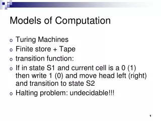
4. Recursive and Recursively Enumerable DEF: A language is recursively enumerableif it is recognized by some Turing Machine. A language is recursive if it is decided by some Turing Machine. The terminology “recursively enumerable” comes from another TM model: a TM which never halts (when describing an infinite language) and writes one string of the language at a time on an auxiliary printer.

5. Recursive EnumeratorExample For example, at some point, the print-out of a recursive enumerator for pal might look like: • (empty string) • a • b • aa • bb • aba • bab • aaa • bbb

6. Recursive EnumeratorExample Recursive-enumerators are equivalent to TM recognizers because of the following intuition: • Enumerator  TM: Given any input, you could simulate the enumerator. If the input ever appears on the list, accept. • TM  Enumerator: Start with an enumerator for S* and compose with the TM. Dovetail (i.e. multithread) trying to accept each element on the list. If any string accepted, write on enumerator’s output list. See Sipser p. 140–141 for further details.

7. Equivalence of k-tape vs. 1-tape The argument that k-tape TM’s are universal, is fairly convincing. After all, the computers we use daily split their memory into several locations: RAM, Hard-Disc, Floppy, CD-ROM. It is plausible that each memory unit could be simulated by a separate tape. The following theorem implies that the computer could still function fully (though probably with a loss of efficiency) if all the memory was merged onto a single tape:

8. Equivalence of k-tape vs. 1-tape THM: Every k-tape TM can be simulated by a 1-tape TM, and vice versa. Proof. It’s clear that every 1-tape TM can be simulated by a k-tape TM. Simply ignore tapes no. 2 through k. On the other hand, to show that any k-tape TM can be simulated by a 1-tape TM, we’ll show two parts: • Any k-tape TM can be simulated by a 2k-track TM. • Any k-track TM can be simulated by a 1-tape TM.

9. k-track TM’s A k-track machine contains a tape whose cells are broken into k vertical sub-cells. As opposed to k-tape machines, there is only one reading head1, but it may read all k tracks and base its actions on these values. EG. A 2-tape machine: vs. a 2-track machine:

10. k-track TM’s A k-track machine contains a tape whose cells are broken into k vertical sub-cells. As opposed to k-tape machines, there is only one reading head1, but it may read all k tracks and base its actions on these values. EG. A 2-tape machine: vs. a 2-track machine:

11. 2k-tracks Simulating k-tapes We can simulate any k-tape TM by a k-track TM as follows: • Each tape of the k-tape TM is represented by one track. • Each track representing a tape, is underneath a track which consists of all blanks, except for a single X which tells us which cells of the k-tape TM are active:

12. 2k-tracks Simulating k-tapes For each move of k-tape TM, the 2k-track TM sweeps to right and then to left. • During right-sweep, 2k-track TM notes the current state of the k-tape machine as well as the symbols read by each head, keeping this information in its finite control. Head back when passed all X’s. • During the left-sweep, every X encountered causes corresponding track active cell to change in accordance to the memorized configuration of the k-tape machine. EG:

13. 2k-tracks Simulating k-tapes Corresponding simulation sequence: Notable: k-tape TM transition

14. 2k-tracks Simulating k-tapes Corresponding simulation sequence: Notable: k-tape TM transition

15. 2k-tracks Simulating k-tapes Corresponding simulation sequence: Notable: k-tape TM transition

16. 2k-tracks Simulating k-tapes Corresponding simulation sequence: Notable: k-tape TM transition

17. 2k-tracks Simulating k-tapes Corresponding simulation sequence: Notable: k-tape TM transition

18. 2k-tracks Simulating k-tapes Corresponding simulation sequence: Notable: 2nd head reads  k-tape TM transition

19. 2k-tracks Simulating k-tapes Corresponding simulation sequence: Notable: k-tape TM transition

20. 2k-tracks Simulating k-tapes Corresponding simulation sequence: Notable: 1st head reads 1 passed all X’s! k-tape TM transition

21. 2k-tracks Simulating k-tapes Corresponding simulation sequence: Notable: 2nd phase, on 1st tape: 13,R k-tape TM transition

22. 2k-tracks Simulating k-tapes Corresponding simulation sequence: Notable: 2nd phase, on 1st tape: 13,R k-tape TM transition

23. 2k-tracks Simulating k-tapes Corresponding simulation sequence: Notable: k-tape TM transition

24. 2k-tracks Simulating k-tapes Corresponding simulation sequence: Notable: on 2nd tape: 2,L k-tape TM transition

25. 2k-tracks Simulating k-tapes Corresponding simulation sequence: Notable: on 2nd tape: 2,L k-tape TM transition

26. 2k-tracks Simulating k-tapes Corresponding simulation sequence: Notable: on 2nd tape: 2,L k-tape TM transition

27. 2k-tracks Simulating k-tapes Corresponding simulation sequence: Notable: k-tape TM transition

28. 2k-tracks Simulating k-tapes Corresponding simulation sequence: Notable: k-tape TM transition

29. 2k-tracks Simulating k-tapes Corresponding simulation sequence: Notable: ready for next k-tape TM transition k-tape TM transition

30. 1 tape simulating k-tracks Finally, convert the 2k-track machine to a single tape machine. In a sense, we are already done, as there is only one head. Q: How can the information about a column of tracks be recorded by a single cell?

31. 1 tape simulating k-tracks A: Just expand the tape alphabet G! In this case, the expanded tape alphabet would consist of 4-tuples, and the 4-tuple (,1,X,) would represent the column on the right. Thus a k-track TM is already a 1-tape TM if we look at it the right way. No further modifications are necessary. This complete the simulation of k-tape TM’s by 1-tape TM’s. 

32. Determinizing NTM’s THM: Every non-deterministic TM recognizer (resp. decider) can be converted to an equivalent deterministic TM recognizer (resp. decider). The idea of the proof is as follows: • Simulate the NTM by a deterministic 3-tape TM. • Previous result guarantees that can then convert to a 1-tape deterministic TM.

33. Determinizing NTM’s Consider the following NTM decider for (ab)*b(ab): To see if a string is accepted, we need to look if any computation branches lead to a configuration containing the state “3”: a|bR L bR a|bR 0 1 2 3

34. Determinizing NTM’s a|bR ababa is accepted. L bR a|bR 0 1 2 3 0ababa a0baba ab0aba ab1aba aba0ba aba2ba crash abab0a abab1a ababa0 ababa2 crash abab3a

35. Determinizing NTM’s a|bR While abab should be rejected: Q: How can you turn tree into an algorithm? L bR a|bR 0 1 2 3 0abab a0bab ab0ab ab1ab aba0b aba2b crash abab0 abab1 crash crash

36. Determinizing NTM’s A: Construct the computation tree of the TM from starting configuration. Just see if an accept configuration occurs on some branch. Q: Breadth first search or depth first search?

37. Determinizing NTM’s A: Breadth first search! It the NTM has infinite loops, could get caught on an infinite branch using depth first search. On the other hand, since each node has finitely many children, a BFS is guaranteed to reach an accept configuration, if it exists.

38. Determinizing NTM’s Construct BFS computation tree: • 3-tape TM is used • First tape read only, contains input • Second tape simulates computation on particular branch up to some depth • Last tape contains branching instructions for current simulated branch of computation

39. Determinizing NTM’sBranching Instructions 0ababa 0 In this example, the computation tree was binary, as at most two choices at each step. Denote the first choice by 0, and the second by 1 obtaining unique branch id’s: a0baba 0 1 ab0aba ab1aba 0 0 aba0ba aba2ba 0 1 010 crash abab0a abab1a 0 0 ababa0 ababa2 00000 0 crash abab3a 000100

40. Determinizing NTM’sBranching Instructions BFS would proceed as follows: • Try 0, if accept configuration, accept. • Try 1, if accept configuration, accept. • Try 00, if accept configuration, accept. • Try 01, if accept configuration, accept. • Try 10, if accept configuration, accept. • Try 11, if accept configuration, accept. • Try 000, if accept configuration, accept. • Try 001, if accept configuration, accept. … In our case, we would finally accept at: • Try 000100, ACCEPT!

41. Determinizing NTM’s For recognizers, nothing needs to be modified. For deciders. König’s Infinity Lemma implies that computation tree is actually finite for every input, so can construct whole tree so can tell when a string is rejected after reading entire tree.