Download
1 / 48
480 likes | 497 Vues
Ad Hoc Wireless Routing CS 218- Fall 2003. Wireless multihop routing challenges Review of conventional routing schemes Proactive wireless routing Hierarchical routing Reactive (on demand) wireless routing Geographic routing. Readings.

E N D
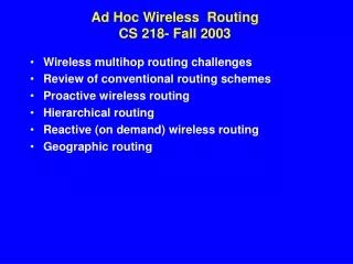
Ad Hoc Wireless RoutingCS 218- Fall 2003 • Wireless multihop routing challenges • Review of conventional routing schemes • Proactive wireless routing • Hierarchical routing • Reactive (on demand) wireless routing • Geographic routing
Readings • G. Pei, M. Gerla, and X. Hong, " LANMAR: Landmark Routing for Large Scale Wireless Ad Hoc Networks with Group Mobility," In Proceedings of IEEE/ACM MobiHOC 2000, Boston, MA, Aug. 2000. • R. Ogier, F. Templin, M. Lewis, " Topology Dissemination Based on Reverse-Path Forwarding (TBRPF) ," IETF Internet Draft , July 28 2003. • Thomas Clausen, Philippe Jacquet, " Optimized Link State Routing Protocol (OLSR) ," IETF Internet Draft , July 3 2003. • X. Hong, K. Xu, and M. Gerla, " Scalable Routing Protocols for Mobile Ad Hoc Networks " IEEE Network Magazine, July-Aug, 2002, pp. 11-21
Wireless multihop routing challenges • mobility • need to scale to large numbers (100’s to 1000's) • unreliable radio channel (fading, external interference, etc) • limited bandwidth • limited power • need to support multimedia applications (QoS)
Proposed ad hoc Routing Approaches • Conventional wired-type schemes (global routing, proactive): • Distance Vector; Link State • Hierarchical routing: • Scalable schemes: • Fisheye, OLSR, TBRPF, Landmark Routing • On- Demand, reactive routing: • Source routing; backward learning • Geo-routing: • etc • clustering • Motion assisted routing
Conventional wired routing limitations • Distance Vector (eg, Bellman-Ford, DSDV): • routing control O/H linearly increasing with net size • convergence problems (count to infinity); potential loops • Link State (eg, OSPF): • link update flooding O/H caused by frequent topology changes CONVENTIONAL ROUTING DOES NOT SCALE TO SIZE AND MOBILITY
Distance Vector 0 Routing table at node 5 : 1 3 2 4 Tables grow linearly with # nodes Control O/H grows with mobility and size 5
1 Link State Routing • At node 5, based on the link state pkts, topology table is constructed: • Dijkstra’s Algorithm can then be used for the shortest path 0 {1} {0,2,3} {1,4} 3 2 {1,4,5} 4 {2,3,5} 5 {2,4}
Topology reduction schemes– OLSR and TBRPF • The link state protocol explodes because of Link State update overhead • Question: how can we reduce the O/H? • (1) if the network is “dense”, use fewer forwarding nodes • (2) if the network is dense, advertise only a subset of the links • Two leading IETF Link State schemes enhance scalability in large scale networks: • OLSR : Optimal Link State Routing • TBRPF: Topology Broadcast Reverse Path Routing
OLSR Overview • In LSR protocol a lot of control messages unnecessary duplicated • In OLSR only a subset of neighbors Multipoint Relay Selectors retransmit control messages: • Reduce size of control message; • Minimize flooding • Other advantages (the same as for LSR): • As stable as LSR protocol; • Proactive protocol; • Does not depend upon any central entity; • Tolerates loss of control messages; • Supports nodes mobility.
Multipoint Relays (MPR) • Designed to reduce duplicate retransmission in the same region • Each node chooses a set of nodes (MPR Selectors) in the neighborhood, which will retransmit its packets. • The other nodes in the neighborhood receive and process the packet, but do not retransmit it • MPR Selectors of node N - MPR(N) • - one-hop neighbors of N • - Set of MPR’s is able to transmit to all • two-hop neighbors • Link between node and it’s MPR is bidirectional.
11 retransmission to diffuse a message up to 3 hops 24 retransmissions to diffuse a message up to 3 hops Retransmission node Retransmission node Optimized Link state routing (OLSR)
Multipoint Relays (MPR) cont. • Every node keeps a table of routes to all known destination through its MPR nodes • Every node periodically broadcasts list of its MPR Selectors (instead of the whole list of neighbors). • Upon receipt of MPR information each node recalculates and updates routes to each known destination • Route is a sequence of hops through MPR’s from source to destination • All the routes are bidirectional
Neighbor sensing • Each node periodically broadcasts Hello message: • List of neighbors with bidirectional link • List of other known neighbors. (If node sees itself in this list it adds the sender to neighbors with bidirectional link) • Hello messages permit each node to learn topology up to 2 hops • Based on Hello messages each node selects its set of MPR’s
Example of neighbor table Two-hop neighbors One-hop neighbors Also every entry in the table has a timestamp, after which the entry in not valid
MPR Selection • MPR set is calculated in a manner to contain a subset of one hop neighbors, which cover all the two hop neighbors • MPR set need not to be optimal (Moreover it is a hard problem to find an optimal set!) • The algorithm of selecting MPR is not presented in this paper. • MPR is recalculated if detected a change in one-hop or two-hops neighborhood topology • MPR Selector Table contains addresses of neighbors, who selected the node as MPR • MPR Selector Table has a Sequence Number, which is incremented after every MPR update.
Conclusions • OLSR is a proactive protocol • Suitable for applications, which does not allow long time delays • Adapted for dense network (reduces control traffic overhead)
TBRPF Overview • TBRPF (Topology Broadcast Based on Reverse-Path Forwarding) is a proactive, link-state protocol. • TBRPF-FT (Full Topology) • Each node is provided with the state of every link in the network. • Useful for sparse topologies and when full topology information is needed. • TBRPF-PT (Partial Topology): • Each node is provided with only enough information to compute min-hop paths to all other nodes. • Useful for dense topologies. • This presentation will focus on TBRPF-PT.
TBRPF Overview (cont.) • TBRPF uses a parent-child relationship to maintain a dynamically changing min-hop broadcast tree rooted at each update source (advertising router). The parent p(u) for source u is the next node on the min-hop path to source u. A NEW PARENT message is sent when p(u) changes. • A node forwards the updates emanating from source u only for links (u,v) such that node v is not a leaf of the broadcast tree rooted at node u, i.e., such that children(u) is nonempty. • A node reports only updates for links in the node’s source tree (consisting of min-hop paths to all other nodes). • Thus (in PT) each node reports only links in part of its source tree, called the reportable subtree. In dense topologies, most nodes will report only a small part of their source tree.
Overview of TBRPF-PT • Each node computes its source tree (providing min-hop paths to all neighbors) based on partial topology information received from its neighbors, using Dijkstra’s algorithm • Each node reports only part of its source tree, called its reportable subtree, defined as the links (u,v) of its source tree such that children(u) is nonempty. • DifferentialTREE UPDATEs are transmitted (e.g., every 1 sec with HELLOs), which report changes (i.e., additions and deletions), to its reportable subtree. (This ensures fast propagation of changes to all nodes affected by the change.) • Periodic TREE UPDATEs are transmitted (e.g., every 5 sec), which describe the entire reportable subtree. (This informs new neighbors, and neighbors that missed a previous update, of the reportable subtree.)
Overview of TBRPF-PT (cont.) • Message types: • TREE UPDATE: Reports differential and periodic updates for the reportable source tree. • NEW PARENT: Selects a new parent/MPR for a source that is 2 hops away. In this way a child selects the MPR (unlike OLSR). • DELETE PARENT: Sent by the parent/MPR source to delete redundant parents/MPRs. They are ACKed by TREE UPDATE messages (which report the link to the parent/MPR source).
Example illustrating TBRPF-PT Node 1 selects node 2 as parent for sources 7, 3, and 11. 9 6 7 8 5 4 2 3 1 13 As a result, node 2 reports its entire source tree, while nodes 6 and 10 report only a small part of their trees. 12 10 11 15 14 Node 2’s reportable subtree Node 6’s reportable subtree Node 10’s reportable subtree
Example illustrating TBRPF-PT Link (12, 15) breaks, so node 2 adds link (14, 15) to its source tree. 9 6 7 8 5 4 2 3 1 13 Node 2 reports the addition of link (14, 15), since it is on node 2’s reportable subtree. 12 10 11 BREAK 15 14 Node 2’s reportable subtree “Add (14, 15)” reported by node 2. Implicit delete for (12, 15). Node 6’s reportable subtree Node 10’s reportable subtree
Example illustrating TBRPF-PT 9 The path computed by node 1 to node 5 is shown in pale blue. 6 7 8 5 4 2 3 1 13 12 Node 1 forwards packets with dest 5 to node 2. 10 11 15 14 Node 2’s reportable subtree Node 6’s reportable subtree Node 10’s reportable subtree
Example illustrating TBRPF-PT 9 Link (1,2) breaks. Node 1 immediately reroutes thru node 6 6 7 8 5 4 2 3 1 BREAK 13 12 10 and sends a New Parent msg, adding node 6 as parent for source 3. 11 15 14 Node 2’s reportable subtree Node 6’s reportable subtree Node 10’s reportable subtree
Example illustrating TBRPF-PT 9 Nodes 6 and 10 add links to their reportable subtrees. 6 7 8 5 4 2 3 1 BREAK 13 12 10 Node 2 no longer reports these links, after node 3 deletes node 2 as parent. 11 15 14 Node 2’s reportable subtree Node 6’s reportable subtree Node 10’s reportable subtree
Comparison to Other Link-State Protocols • In STAR, each node reports its entire source tree to neighbors (which is redundant since the source trees of two neighboring nodes can overlap considerably), while in TBRPF-PT each node reports only part of its source tree. • In DSDV each node reports its distances to all destinations, i.e., O(|V|) numbers, while in TBRPF-PT, each node reports less than this, since it reports only part of its source tree. • Each node reports fewer links in TBRPF-PT than in OLSR, since the reportable subtree reported by TBRPF-PT is a subset of the MPR links reported by OLSR.
Benefit of child selection of MPRs • In the example below, if link (i,j) fails due to a link-layer indication, then in TBRPF-PT, node i will immediately select j’ as the new MPR. • In OLSR, node i is not allowed to reroute through node j’ until it knows j’ is an MPR. This can take up to 19 seconds (assuming no messages fail): 6 sec for node j to detect that the link failed + 6 sec for node k to learn that the link failed + 2 sec for node k to select j’ as the new MPR + 5 sec for node j’ to generate a TC message reporting its MPR link to k. j (MPR) u k failure i source child j’
Control Traffic vs. Number of Nodes(for previous version of TBRPF-PT) For 80 nodes, PT generated 90% less control traffic than Flooding, and 38% less than FT.
Where do we stand? • OLSR and TBRPF can dramatically reduce the “state” sent out on update messages • They are very effective in “dense” networks. • However, the state still grows with O(N) • Neither of the above schemes can handle large scale nets from 10’s to thousands of nodes • What to do?
APPROACH: use hierarchical routing to reduce table size and table update overhead Proposed hierarchical schemes include: • Hierarchical State Routing • Fisheye (implicit hierarchy induced by "scope") • Zone routing (hybrid scheme) • Landmark Routing
Hierarchical State Routing (HSR) • Loose hierarchical routing in Internet • Main challenge in ad hoc nets: maintain/update the hierarchical partitions in the face of mobility • Solution: distinguish between “physical” partitions and “logical” grouping • physical partitions are based on geographical proximity • logical grouping is based on functional affinity between nodes (e.g., tanks of same battalion, students of same class) • Physical partitions enable reduction of routing overhead • Logical groupings enable efficient location management strategies using Home Agent concepts
3 1 Level = 2 2 3 1 Level = 1 4 2 8 9 6 3 1 Level = 0 10 11 7 5 4 HSR - physical multilevel partitions HSR table at node 5: DestID 1 6 7 <1-2-> <1-4-> <3--> Path 5-1 5-1-6 5-7 5-1-6 5-7 5-7 HID(5): <1-1-5> HID(6): <3-2-6> Hierarchical addresses (MAC addresses)
HSR - logical partitions and location management • Logical (IP like) type address <subnet,host> • Each subnet corresponds to a particular user group (e.g., tank battalion in the battlefield, search team in a search and rescue operation, etc) • logical subnet spans several physical clusters • Nodes in same subnet tend to have common mobility characteristic (i.e., locality) • logical address is totally distinct from MAC address
HSR - logical partitions and location management (cont’d) • Each subnetwork has at least one Home Agent to manage membership • Each member of the subnet registers its own hierarchical address with Home Agent • periodical/event driven registration; stale addresses are timed out by Home Agent • Home Agent hierarchical addresses propagated via routing tables; or queried at a Name Server • After the source learns the destination’s hierarchical address, it uses it in future packets
Fisheye State Routing • Topology data base at each node - similar to link state (e.g., OSPF) • Routing information is periodically exchanged with neighbors only ( “Global” State Routing) • similar to distance vector, but exchange entire topo matrix • Routing update frequency decreases with distance to destination • Higher frequency updates within a close zone and lower frequency updates to a remote zone • Highly accurate routing information about the immediate neighborhood of a node; progressively less detail for areas further away from the node
2 8 3 5 9 1 9 4 6 Hop=1 7 10 12 13 Hop=2 19 18 21 11 Hop>2 15 22 36 14 23 17 16 20 29 35 27 25 24 26 28 34 30 32 31 Scope of Fisheye
Message Reduction in FSR LST HOP 0 LST HOP 0:{1} 1:{0,2,3} 2:{5,1,4} 3:{1,4} 4:{5,2,3} 5:{2,4} 1 0 1 1 2 2 0:{1} 1:{0,2,3} 2:{5,1,4} 3:{1,4} 4:{5,2,3} 5:{2,4} 2 1 2 0 1 2 1 3 LST HOP 2 0:{1} 1:{0,2,3} 2:{5,1,4} 3:{1,4} 4:{5,2,3} 5:{2,4} 2 2 1 1 0 1 4 5
Logical Subnet Landmark Our Solution: Landmark Routing (LANMAR) • Key insight: nodes move in teams/swarms • Each team is mapped into a logical subnet • IP-like Node address = <subnet, host> • Address compatible with IPv6 • Team leader (Landmark) elected in each group
48 bits 48 bits 16 bits 16 bits 64 bits 64 bits LANMAR Addressing in IPv6 • “Limited-Scope” IPv6 address format proposed in IETF Internet draft (<draft-templin-lsareqts-00.txt) • LANMAR addressing: Keep the unique network ID field as it is. Use the middle 16 bits to store group IDs. Node ID Group-ID Network ID Subnet Mask 00000000 … 0000000 0000 … 000 11 … 11
Logical Subnet Landmark LANMAR Overview (cont) • Three main components in LANMAR: • (1) “local ” routing algorithm that keeps accurate routes within local scope < k hops (e.g., Distance Vector) • (2) Landmark selection for each logical group • (3) Landmark routes advertised to all nodes
Logical Subnet Landmark Landmark Routing Overview (cont) • Packet Forwarding: • A packet to “local” destination is routed directly using local tables • A packet to remote destination is routed to corresponding Landmark • Once the packet is “in sight” of Landmark, the direct route is found in local tables. • Landmarks form a two level logical hierarchy that reduces routing O/H
Link Overhead of LANMAR • Dramatic O/H reduction from linear to O(N) to O (sqrtN)
How does LANMAR compare with MANET routing schemes? We compare: • MANET routing schemes: DSDV, TBRPF and FSR; and (b) same MANET schemes, BUT used for local scope only; LANMAR used for long paths.
LANMAR enhances existing routing alg.s LANMAR-DSDV LANMAR-TBRPF LANMAR-FSR TBRPF FSR DSDV ( scope = 2, # of group increases)
Backbone Network and LANMAR • Why a Backbone “physical” hierarchy? • To improve coverage, scalability and reduce hop delays • Backbone deployment • automatic placement: Relocate backbone nodes from dense to sparse regions (using repulsive forces) • Key result: LANMAR automatically adjusts to Backbone • Combines low routing O/H (LANMARK logical hierarchy) + low hop distance and high bandwidth (Backbone physical hierarchy)
Backbone Node Deployment • Deployment algorithm • Assumption: Backbone nodes know their position (from GPS) • Each BN broadcasts its position periodically via scoped flooding. • Let the distance between x and y = Dxy. We define the repulsive force between them where A is a constant. • Vector sum of repulsive forces from neighbors determines direction and speed of motion