Download
1 / 87
870 likes | 1.08k Vues
Introduction to Valuation Bond Valuation. Financial Management P.V. Viswanath For a First course in Finance. Lesson Objectives. To look at the difference between economics and finance To introduce the notion of future dollars as traded goods. To introduce the price of future dollars

E N D
Introduction to ValuationBond Valuation Financial Management P.V. Viswanath For a First course in Finance
Lesson Objectives • To look at the difference between economics and finance • To introduce the notion of future dollars as traded goods. • To introduce the price of future dollars • To relate the price of money to interest rates. • To use these rates to price Treasury securities • To introduce the notion of arbitrage P.V. Viswanath
Absolute and Relative Pricing • In economics, we tend to price goods and assets by considering the factors affecting the supply and demand for them. • The number of goods and assets are very many. Each of them is different in some way or another from the other. • Computing the price of one good does not allow us to price another good, except to the extent that other goods are substitutes or complements for the first good. • In finance, the number of assets can be reasonably characterized in terms of a smaller number of basic characteristics. • Hence most assets can, to a first approximation be priced by considering them as combinations of more fundamental assets. P.V. Viswanath
The Fundamentals of Economics • One of the issues that economics analyzes is the determination of prices of goods. • For example, what determines the price of eggs? • We have a supply curve – that is, a schedule of quantities of eggs that their current possessors would be willing to sell and the prices at which they would be willing to sell them. • The higher the price, the more they’d be willing to sell. P.V. Viswanath
S The Supply Curve Price ($ per unit) Quantityof Eggs P.V. Viswanath
The Demand Curve • We can also imagine the different amounts of eggs that people would be willing to buy and the prices at which they would buy those quantities. • The lower the price, the more would be demanded. P.V. Viswanath
D The Demand Curve Price ($ per unit) Quantity of Eggs P.V. Viswanath
S The curves intersect at equilibrium, or market- clearing, price. At P0the quantity supplied is equal to the quantity demanded at Q0 . P0 D Q0 The Determination of the Price of Eggs Price ($ per unit) Quantityof Eggs P.V. Viswanath
Economics and Finance • Finance, like Economics, is interested in the prices of goods. • But the goods that financial analysts are interested in, are quite different. • As you might imagine, financial economists are interested in money (or purchasing power) and in the price of money. • But what does it mean to talk about the price of money? In what currency would you pay to acquire money? P.V. Viswanath
Money and Time • The answer is that access to resources today is not the same as access to resources tomorrow – that is, money available today is not the same as money available tomorrow. • You can buy something today only if you have the money to buy it with today. Having access to money, which will be available tomorrow won’t allow you to necessarily buy things today! • This means that we can talk of different kinds of money. • And, denoting time by the subscript t, we can talk of the price of time 1 (tomorrow) money in terms of time 0 (today) money. P.V. Viswanath
More on the price of money • Let’s assume that all prices are denominated in t=0 dollars (today’s money). • Then, just as we might say that the price of a book is $10, the price of a subway token is $2 and the price of a cup of Starbucks coffee is $3.50, we could also say • The price of a t=1 dollar is $0.90, the price of a t=2 dollar is $0.7831 and the price of a t=3 dollar is $0.675. P.V. Viswanath
The price of coffee, said differently • This might sound a little strange to you, but let’s put it slightly differently. • Going back to a cup of coffee, we said its price was $3.50, but if we know that $3.50 = €1, we could equally well say that the price of a book is €1. • Then even if we were all in the US and Starbucks only accepted US dollars, there would be no problem if Starbucks had its price list denominated in euros. P.V. Viswanath
More ways to price coffee • Let’s take this further. • Suppose Starbucks required everybody to play the following game in order to figure out the price of its offering. • Suppose they took the actual dollar price of a coffee multiplied it by 2 and added 3 to it and called it java units (J). • A cup of coffee that normally cost $3.5 would be listed as costing 10J. • Then if we saw a cappuccino listed at 13J, we would simply subtract 3 to get 10, then divide by 2 to get a price of $5. • It would be a little weird, but nothing substantive would change. P.V. Viswanath
Rates • So now, let’s go back to the price of money: we said that the price of a t=1 dollar was $0.90, and that the price of a t=2 dollar was $0.7831. • Now clearly the price of a t=1 dollar, which is $0.90 today, will rise to $1 at t=1. • Hence providing today’s price of a t=1 dollar is equivalent to providing the rate of change of the price over the coming period. • I have exactly the same information in each case. • This rate of change is also my rate of return over the next year if I buy a t=1 dollar, today, and is also known as the interest rate. • In our example, this works out to (1-0.90)/0.90 or 11.11% P.V. Viswanath
Rates • What about the price of a t=2 dollar, which we said was $0.7831? • Once again, the price of this t=2 dollar would be $1 at t=2 (in t=2 dollars, of course). • We could compute the gross return on this investment, in the same way, as 1/0.7831 = 1.277 or a return of 27.70%. • But this is a return over two periods, and we cannot compare it directly to the 11.11% that we computed earlier. • The solution to this problem is to annualize the two-period return P.V. Viswanath
Computing Annualized Rates • We computed the return on buying a t=2 dollar at 27.70%. • Suppose the one-period return on this is r%; that is, the return from holding this t=2 dollar from now until t=1 is r%. Then, every dollar invested in this specialized investment could be sold at $(1+r) at t=1. • Now, if we assume the return on this t=2 dollar if held from t=1 to t=2 is also r%, then the $(1+r) value of our outlay of one t=0 dollar in this investment would be $(1+r)(1+r) or (1+r)2. • But we already know from our return computation, that this is exactly 1.277 (that is 1 plus the 27.7%). • Hence we equate (1+r)2 to 1.277 and solve for r. P.V. Viswanath
Annualized Rates • This involves simply taking the square-root of 1.277, which is 13%. • Of course, we won’t get exactly 13% in each of the two periods. • The 13% rate is, rather, a sort of average return over the two periods, that results in a 27.7% over the two years. • We can now take $0.675, the price of a t=3 dollar and also convert it to a rate of return. • In this case, we take the cube root of (1/0.675), which works out 14% P.V. Viswanath
Yield to maturity • So now we have the current prices of t=1, t=2, and t=3 dollars, or $0.90, $0.7831 and $0.675 respectively. • Alternatively, the information in these prices could also be presented as rates of return, which in our case are 11.11%, 13% and 14% respectively. • These rates are also called yields-to-maturity. • Yields-to-maturity, in general, are the annualized total returns that you would get if you held a particular financial instrument to maturity. • In this case, the returns each year are only from price appreciation, while in other cases, there may be annual cash payments received by the investor, as well. P.V. Viswanath
Using the rates • We have assumed, up to this point, that purchasing a t=1 dollar is riskless. That is, the person who sold us the t=1 dollar today, in return for the $0.90, would, in fact, pay us $1 at time t=1. • We will continue with this assumption, for now. • Note, as well that buying a t=1 dollar is equivalent to lending money for one period, while selling a t=1 dollar is equivalent to borrowing money for 1 period. • A bond is precisely a promise to pay its holder some combination of future dollars. • Corporations, governments and other entities who need funds for the continuing operations issue, that is sell, such bonds. P.V. Viswanath
Treasury Bonds • Consider now a bond issued by the Treasury Department, which essentially acts as banker for the Federal Government. • These bonds, or promises to pay are considered default-free, i.e. we fully expect the Treasury to live up to its promises. • We can, therefore, evaluate and price these Treasury or T-bonds using the “risk-free” yields that we established before. • This need not be true of other governmental institutions, such as municipalities, such as the City of New York or Federal agencies such as PATH – the Port Authority of New York and New Jersey. P.V. Viswanath
Treasury Bonds • On Feb. 29th 2008, the Treasury issued a 2% note with a maturity date of February 28, 2010 with a face value of $1000, which was sold at auction. • The price paid by the lowest bidder was 99.912254% of face value. • This means that the buyer of this bond would get every six months 1% (half of 2%) of the face value, which in this case works out to $10. • In addition, on Feb. 28, 2010, the buyer would get $1000. P.V. Viswanath
Terminology • The maturity of this bond is 2 years. • The coupon rate on this bond is 2% • The face value of this bond is $1000 • The price paid for this bond is $999.123 • The yield-to-maturity obtained by this buyer is 2.045%, i.e. the average rate of return for this buyer if s/he held it to maturity. P.V. Viswanath
Pricing this bond • Let’s assume for now, that we do not know the price of this bond. How can we price this bond? • What we do know is that a holder of this bond would receive $10 in 6 months, another $10 in 1 year, $10 again in 1.5 years and $1010 in 2 years. • We also know that a 6-month T-bill issued on Feb. 21, 2008 sold for 98.968667. • A T-bill is a promise to pay money 6 months in the future. With the given price then, a buyer would get a 1.042% return for those 6 months. • This is often annualized by multiplying by 2 to get a bond-equivalent yield of 2.084%. • We also know that yields of bonds generally are higher for higher maturities. P.V. Viswanath
Yield Curves for Feb. 1-12, 2008 P.V. Viswanath
Yield Curves for Feb. 1-12, 2008 P.V. Viswanath
Pricing a Treasury bond • Suppose we believe that the current environment of uncertainty will continue. • We might believe that investors will be even more unwilling to invest in securities that have any default risk. • In that case, they will be willing to buy Treasury securities at lower yields. • We use this to estimate current bond-equivalent yields. • Suppose we estimate the current bond-equivalent yields for 6-month money, 1 year money, 18-month money and 2 year money as 2.07%, 2.1%, 2.11% and 2.14%. P.V. Viswanath
Discounting • Keeping in mind that what we have are bond-equivalent yields, i.e. yields computed on a six-monthly basis and then doubling to get the annual yield, we will compute the current prices of future dollars. • To do this, we need to employ a procedure called discounting. • Suppose the required risk-free rate of return on future dollars is 4% per period. • Now, if I have a certain, default-free promise of $200 in 3 periods, what is the value of this promise today? P.V. Viswanath
Discounting • We know the value at t=3 of this promise would be exactly 200. • The value at t=2of the promise would have to be such that would yield a return of exactly 4% over the last period, i.e. from t=2 to t=4. • Suppose the required value is $S. Then, we would need (200-S)/S = 1.04. • Solving this equation, we find S = 200/1.04. • What would the value at t=1 be? • Applying the same principle, we see that it must be S/1.04 or 200/1.042. • Analogously, we can see that the value at t=0 of a promise to pay $200 in n periods is 200/(1.04)n. P.V. Viswanath
Pricing the 2-yr T-bond • Coming back to our T-bond, the annualized yield on 6-month money is 2.07%; hence the six-month yield is 2.07/2 or 1.035%. • Hence a promised dollar-payment at t = 0.5 would sell today for 1/1.01035 or $0.989756 today. • The annualized yield on 1-year money is 2.1%; hence the six-month yield is 2.10/2 = 1.05%. • Hence a promised dollar-payment at t=1 would sell today for 1/1.01052 = 0.979326. P.V. Viswanath
Pricing the 2-yr T-bond • The annualized yield on 1.5 year money is 2.11; hence the six-month yield is 2.11/2 = 1.055%. • Hence the price today of a promised dollar-payment at t=1.5 is 1/1.010553 = 0.96901, using the discounting method. • The annualized bond-equivalent yield on 2-year money is 2.14%. • The price today of a promised dollar-payment at t=2 is 1/1.01074 = 0.95832 P.V. Viswanath
Pricing the 2-yr T-bond • So now we know that our bond pays $10 in 6 months, another $10 in 1 year, $10 again in 1.5 years and $1010 in 2 years. • We also know that one dollar promised for each of those dates is worth, today, $0.989756, $ 0.979326, $ 0.96901 and $ 0.95832 respectively. • Our bond, therefore, must sell for 10(0.989756) + 10(0.979326) + 10(0.96901) + 1010(0.95832) = $997.28. P.V. Viswanath
Arbitrage • What we have done is to treat our 2 year 2% coupon bond as a portfolio of four other zero-coupon bonds and then priced it as the sum of the values of those zero-coupon bonds. • But what will guarantee that this price equality will hold? • Here’s where the efficient functioning of markets comes into play. • A process called arbitrage ensures that the price of a combination of other financial securities does not deviate too much from the price implied the prices of those other securities. P.V. Viswanath
Arbitrage • Suppose, for example that our two-year bond sold for $996. • Then a bond trader could buy a bond at this price, then, himself, issue the corresponding four zero-coupon bonds and sell them at their market prices. • He would then end up with a profit of $1.28 per bond. • If the bond sold for, say, $998, he could buy the zero-coupon bonds and then create a “synthetic” coupon bond and sell it at the higher price and make a profit of 998-997.28 or 72 cents per bond. P.V. Viswanath
Relative pricing of financial assets • Consider first riskless financial assets, i.e, assets that are claims on riskless cashflows over time. • Consider a fundamental asset, i, defined by a claim to $1 at time t = i. • There can be T such fundamental assets, corresponding to the t = 1,..,T time units. • Then, any arbitrary riskless financial asset that is a claim to $ci at time i, i = 1,..,T can be considered a portfolio of these T fundamental assets. • Hence, the price, P* of any such asset is related to the prices of these first T fundamental assets. • In fact, the price of this asset would simply be P.V. Viswanath
Relative pricing of risky financial assets • What about risky financial assets? • We can equivalently imagine, for every level of risk, a set of T fundamental risky assets. Then, for any arbitrary risky asset of this level of risk, we can equivalently write: • Of course, this is not entirely satisfactory, because we’d have TxM fundamental assets corresponding to each of M levels of risk. We will come back to this when we talk about the CAPM. • In any case, we need to examine how this pricing is established in the market-place. P.V. Viswanath
Arbitrage and the Law of One Price • Law of One Price: In a competitive market, if two assets generate the same cash (utility) flows, they will be priced the same. • How is this enforced? • If the law is violated – if asset 1 sells for more than asset 2, then investors can make a riskless profit by buying asset 2 and selling it as asset 1! • In practice – we need to take transactions costs into account. • Also, it may be difficult to execute the two transactions at the same time – prices might change in that interval – this introduces some risk. P.V. Viswanath
Exchange Rates and Triangular Arbitrage • Consider the exchange rates reigning at closing on January 30. • The yen/euro rate was 157.87 yen per euro • The euro/$ rate was $1.4835 per euro. • The yen/$ rate was 106.4 yen per dollar. • If we start with a dollar, we can buy 106.4 yen; these can then be used to buy 106.4/157.87 or 0.674 euros, which can, in turn, be used to acquire $0.9998, which is very close to a dollar. P.V. Viswanath
Triangular Currency Arbitrage • Suppose the euro/$ rate had been $1.50 per euro. • Then, it would have been possible to start with one dollar, acquire 0.674 euros, as above, and then get (0.674)(1.5) or $1.011, or a gain of 1.1% on the initial investment of a dollar. • This would imply that the dollar was too cheap, relative to the euro and the yen. • Many traders would attempt to perform the arbitrage discussed above, leading to excess supply of dollars and excess demand for the other currencies. • The net result would be a drop a rise in the price of the dollar vis-à-vis the other currencies, so that the arbitrage trades would no longer be profitable. P.V. Viswanath
Risk Arbitrage • In this case, trading will continue until there are no more riskfree profit opportunities. • Thus, arbitrage can ensure that the sorts of pricing relationships referred to above can be supported in the marketplace, viz: • What if there are still opportunities that will, on average, lead to profit, but the investors intending to benefit from this profit will have to take on some risk? • Presumably investors will trade off the risk against the expected profit so that there will be few of these expected profit opportunities, as well; this brings us to the notion of the informational efficiency of financial markets. P.V. Viswanath
Efficient Markets Hypothesis – EMH • An asset’s current price reflects all available information– this is the EMH. • If it didn’t, there would be an incentive for investors to act on that information. • Suppose, for example, that investors noticed that good news led to stock prices rising slowly over two consecutive days. • This would mean that at the end of the first day, the good news was not all incorporated in the stock price. P.V. Viswanath
Efficient Markets Hypothesis • In this situation, it would be optimal for traders to buy even more of a stock that was noted to be rising on a given day, since the stock would rise more the next day, giving the trader an unusually good chance of making money on the trade. • But if many traders pursue this strategy, the stock price would rise on the first day, itself, and the informational inefficiency would be eliminated. • Empirically, financial markets seem to be reasonably close to being efficient. • This allows us to price financial assets with respect to fundamentals without worrying about deviations from these fundamental prices. P.V. Viswanath
Stock Price Fundamentals • What determines the price of a stock? Or, in other words, why would an investor hold stocks? • The answer is that s/he expects to receive dividends and hopefully benefit from a price increase, as well. • In other words, P0 = PV(D1) + PV(P1) • However what determines P1? • Again, using the previous logic, we must say that it’s the expectation of a dividend in period 2 and hopefully a further price rise. Continuing, in this vein, we see that the stock price must be the sum of the present values of all future dividends. P.V. Viswanath
Dividend Mechanics • Declaration date: The board of directors declares a paymentRecord date: The declared dividends are distributable to shareholders of record on this date.Payment date: The dividend checks are mailed to shareholders of record. • Ex-dividend date: A share of stock becomes ex-dividend on the date the seller is entitled to keep the dividend. At this point, the stock is said to be trading ex-dividend. P.V. Viswanath
Dividend Discount Model • What is the price of a stock on its ex-dividend date? • Using the previous logic, we see that it’s simply • where k is the appropriate discount rate to discount the dividends consistent with their riskiness. • We assume that the one-period ahead discount rate is the same for all periods. That is, we use the same rate to discount D1 to time 0, as we use to discount D2 to time 1. P.V. Viswanath
Gordon Growth Model • If we assume that the dividend is growing at a rate of g% per annum forever, this formula simplifies to: • We see that the price of a stock is higher, the higher the level of dividends, the higher the growth rate of dividends and the lower the required rate of return or the discount rate, k. P.V. Viswanath
Two essential concepts • Cash flows at different points in time cannot be compared and aggregated. All cash flows have to be brought to the same point in time, before comparisons and aggregations are made. • The concept of a Time Line: P.V. Viswanath
Cash Flow Types and Discounting Mechanics • There are five types of cash flows - • simple cash flows, • annuities, • growing annuities • perpetuities and • growing perpetuities P.V. Viswanath
I. Simple Cash Flows • A simple cash flow is a single cash flow in a specified future time period. Cash Flow: CFt ________________________________________|____ Time Period: t • The present value of this cash flow is- PV of Simple Cash Flow = CFt / (1+r)t • The future value of a cash flow is - FV of Simple Cash Flow = CF0 (1+ r)t P.V. Viswanath
Application: The power of compounding - Stocks, Bonds and Bills • Between 1926 and 1998, Ibbotson Associates found that stocks on the average made about 11% a year, while government bonds on average made about 5% a year. • If your holding period is one year,the difference in end-of-period values is small: • Value of $ 100 invested in stocks in one year = $ 111 • Value of $ 100 invested in bonds in one year = $ 105 P.V. Viswanath
Holding Period and Value P.V. Viswanath