
Computer Arithmetic Techniques and Implementations
E N D
Presentation Transcript
Appendix J Computer Arithmetic
Figure J.1 Ripple-carry adder, consisting of n full adders. The carry-out of one full adder is connected to the carry-in of the adder for the next most-significant bit. The carries ripple from the least-significant bit (on the right) to the most-significant bit (on the left).
Figure J.2 Block diagram of (a) multiplier and (b) divider for n-bit unsigned integers. Each multiplication step consists of adding the contents of P to either B or 0 (depending on the low-order bit of A), replacing P with the sum, and then shifting both P and A one bit right. Each division step involves first shifting P and A one bit left, subtracting B from P, and, if the difference is nonnegative, putting it into P. If the difference is nonnegative, the low-order bit of A is set to 1.
Figure J.3 Numerical example of (a) restoring division and (b) nonrestoring division.
Figure J.4 Numerical example of Booth recoding. Multiplication of a = − 6 by b = − 5 to get 30.
Figure J.5 Summary of how various machines handle integer overflow. Both the 8086 and SPARC have an instruction that traps if the V bit is set, so the cost of trapping on overflow is one extra instruction.
Figure J.6 Examples of integer division and integer remainder in various programming languages.
Figure J.7 Format parameters for the IEEE 754 floating-point standard. The first row gives the number of bits in the significand. The blanks are unspecified parameters.
Figure J.8 Representation of special values. When the exponent of a number falls outside the range Emin ≤ e ≤ Emax, then that number has a special interpretation as indicated in the table.
Figure J.9 Examples of rounding a multiplication. Using base 10 and p = 3, parts (a) and (b) illustrate that the result of a multiplication can have either 2p − 1 or 2p digits; hence, the position where a 1 is added when rounding up (just left of the arrow) can vary. Part (c) shows that rounding up can cause a carry-out.
Figure J.10 The two cases of the floating-point multiply algorithm. The top line shows the contents of the P and A registers after multiplying the significands, with p = 6. In case (1), the leading bit is 0, and so the P register must be shifted. In case (2), the leading bit is 1, no shift is required, but both the exponent and the round and sticky bits must be adjusted. The sticky bit is the logical OR of the bits marked s.
Figure J.11 Rules for implementing the IEEE rounding modes. Let S be the magnitude of the preliminary result. Blanks mean that the p most-significant bits of S are the actual result bits. If the condition listed is true, add 1 to the pth most-significant bit of S. The symbols r and s represent the round and sticky bits, while p0 is the pth most-significant bit of S.
Figure J.12 Rules for computing the sign of a sum when the addends have different signs. The swap column refers to swapping the operands in step 1, while the compl column refers to performing a two’s complement in step 4. Blanks are “don’t care.”
Figure J.13 Newton’s iteration for zero finding. If xi is an estimate for a zero of f, then xi + 1 is a better estimate. To compute xi + 1, find the intersection of the x-axis with the tangent line to f at f(xi).
Figure J.14 Pure carry-lookahead circuit for computing the carry-out cn of an n-bit adder.
Figure J.15 First part of carry-lookahead tree. As signals flow from the top to the bottom, various values of P and G are computed.
Figure J.16 Second part of carry-lookahead tree. Signals flow from the bottom to the top, combining with P and G to form the carries.
Figure J.17 Complete carry-lookahead tree adder. This is the combination of Figures J.15 and J.16. The numbers to be added enter at the top, flow to the bottom to combine with c0, and then flow back up to compute the sum bits.
Figure J.18 Carry-skip adder. This is a 20-bit carry-skip adder (n = 20) with each block 4 bits wide (k = 4).
Figure J.19 Combination of CLA and ripple-carry adder. In the top row, carries ripple within each group of four boxes.
Figure J.20 Simple carry-select adder. At the same time that the sum of the low-order 4 bits is being computed, the high-order bits are being computed twice in parallel: once assuming that c4 = 0 and once assuming c4 = 1.
Figure J.21 Carry-select adder. As soon as the carry-out of the rightmost block is known, it is used to select the other sum bits.
Figure J.22 Asymptotic time and space requirements for four different types of adders.
Figure J.23 SRT division of 10002/00112. The quotient bits are shown in bold, using the notation 1 for − 1.
Figure J.24 Carry-save multiplier. Each circle represents a (3,2) adder working independently. At each step, the only bit of P that needs to be shifted is the low-order sum bit.
Figure J.25 Multiples of b to use for radix-4 Booth recoding. For example, if the two low-order bits of the A register are both 1, and the last bit to be shifted out of the A register is 0, then the correct multiple is − b, obtained from the second-to-last row of the table.
Figure J.26 Multiplication of − 7 times − 5 using radix-4 Booth recoding. The column labeled L contains the last bit shifted out the right end of A.
Figure J.27 An array multiplier. The 5-bit number in A is multiplied by b4b3b2b1b0. Part (a) shows the block diagram, (b) shows the inputs to the array, and (c) expands the array to show all the adders.
Figure J.28 Multipass array multiplier. Multiplies two 8-bit numbers with about half the hardware that would be used in a one-pass design like that of Figure J.27. At the end of the second pass, the bits flow into the CPA. The inputs used in the first pass are marked in bold.
Figure J.29 Even/odd array. The first two adders work in parallel. Their results are fed into the third and fourth adders, which also work in parallel, and so on.
Figure J.30 Wallace tree multiplier. An example of a multiply tree that computes a product in 0(log n) steps.
Figure J.31 Signed-digit addition table. The leftmost sum shows that when computing 1 + 1, the sum bit is 0 and the carry bit is 1.
Figure J.32 Quotient selection for radix-2 division. The x-axis represents the ith remainder, which is the quantity in the (P,A) register pair. The y-axis shows the value of the remainder after one additional divide step. Each bar on the right-hand graph gives the range of ri values for which it is permissible to select the associated value of qi.
Figure J.33 Quotient selection for radix-4 division with quotient digits − 2, − 1, 0, 1, 2.
Figure J.34 Quotient digits for radix-4 SRT division with a propagate adder. The top row says that if the high-order 4 bits of b are 10002 = 8, and if the top 6 bits of P are between 1101002 = − 12 and 1110012 = − 7, then − 2 is a valid quotient digit.
Figure J.35 Example of radix-4 SRT division. Division of 149 by 5.
Figure J.36 Summary of the three floating-point chips discussed in this section. The cycle times are for production parts available in June 1989. The cycle counts are for double-precision operations.
Figure J.37 Chip layout for the TI 8847, MIPS R3010, and Weitek 3364. In the left-hand columns are the photomicrographs; the right-hand columns show the corresponding floor plans.