Introduction to (Demand) Forecasting
370 likes | 639 Vues
Learn the role of forecasting, forecasting methods, building models using regression, and confidence intervals for accurate demand forecasts in production planning.

Introduction to (Demand) Forecasting
E N D
Presentation Transcript
Module Outline • The role of forecasting in contemporary production planning frameworks • Basic characterization of the (demand) forecasting problem • Forecasting methods and some selection criteria • A generic approach to quantitative forecasting • Time series-based forecasting • Building causal models through multiple linear regression • Confidence Intervals and their application in forecasting
Forecasting • Def:The process of predicting the values of a certain quantity, Q, over a certain time horizon, T, based on past trends and/or a number of relevant factors. • In the context of OM, the most typically forecasted quantity is future demand(s), but the need of forecasting arises also with respect to other issues, like: • equipment and employee availability • technological forecasts • economic forecasts (e.g., inflation rates, exchange rates, housing starts, etc.) • The time horizon depends on • the nature of the forecasted quantity • the intended use of the forecast
Forecasting future demand • Product/Service demand: The pattern of order arrivals and order quantities evolving over time. • Demand forecasting is based on: • extrapolating to the future past trends observed in the company sales; • understanding the impact of various factors on the company future sales: • market data • strategic plans of the company • technology trends • social/economic/political factors • environmental factors • etc • Rem: The longer the forecasting horizon, the more crucial the impact of the factors listed above.
Demand Patterns • The observed demand is the cumulative result of: • some systematic variation, resulting from the (previously) identified factors, and • a random component, incorporating all the remaining unaccounted effects. • (Demand) forecasting tries to: • identify and characterize the expected systematic variation, as a set of trends: • seasonal: cyclical patterns related to the calendar (e.g., holidays, weather) • cyclical: patterns related to changes of the market size, due to, e.g., economics and politics • business: patterns related to changes in the company market share, due to e.g., marketing activity and competition • product life cycle: patterns reflecting changes to the product life • characterize the variability in the demand randomness
Forecasting Methods • Qualitative (Subjective):Incorporate factors like the forecaster’s intuition, emotions, personal experience, and value system; these methods include: • Jury of executive opinion • Sales force composites • Delphi method • Consumer market surveys • Quantitative (Objective): Employ one or more mathematical models that rely on historical data and/or causal/indicator variables to forecast demand; major methods include: • time series methods: F(t+1) = f (D(t), D(t-1), …) • causal models: F(t+1) = f(X1(t), X2(t), …)
Selecting a Forecasting Method • It should be based on the following considerations: • Forecasting horizon (validity of extrapolating past data) • Availability and quality of data • Lead Times (time pressures) • Cost of forecasting (understanding the value of forecasting accuracy) • Forecasting flexibility (amenability of the model to revision; quite often, a trade-off between filtering out noise and the ability of the model to respond to abrupt and/or drastic changes)
Determine Method • Time Series • Causal Model Collect data: <Ind.Vars; Obs. Dem.> Fit an analytical model to the data: F(t+1) = f(X1, X2,…) Use the model for forecasting future demand Monitor error: e(t+1) = D(t+1)-F(t+1) Model Valid? Applying a Quantitative Forecasting Method - Determine functional form - Estimate parameters - Validate Update Model Parameters Yes No
Time Series-based Forecasting Basic Model: Time Series Model Historical Data Forecasts • Remark: The exact model to be used depends on the expected / • observed trends in the data. • Cases typically considered: • Constant mean series • Series with linear trend • Series with seasonalities (and possibly a linear trend)
A constant mean series The above data points have been sampled from a normal distribution with a mean value equal to 10.0 and a variance equal to 4.0.
The presumed model for the observed data: where is the constant mean of the series and is normally distributed with zero mean and some unknown variance Forecasting constant mean series:The Moving Average model Then, under a Moving Average of Order N model, denoted as MA(N), theestimate of returned at period t, is equal to:
The Moving Average Model:The selection of the model order, N, and its impact on the model accuracy • Some “rules of thumb” for selecting an appropriate value for N: • Smaller values of N give the model more flexibility since it focuses on the more recent observations; this property is useful when the observed series experiences frequent “jumps”. • On the other hand, in case of a stationary series, larger values of N provide more accuracy to the forecasts, since they reduce the variance of the forecasting error; more specifically, defining the forecasting error as: we obtain and
Demonstrating the impact of order N on the model performance In the above plot, the blue series is the original data series, distributed according to N(10,4) for the first 20 points, and N(20,4) for the last 20 points. The magenta series corresponds to the predictions of a MA(5) forecasting model and the yellow series to the predictions of a MA(10) forecasting model. As expected, the MA(5) model adjusts faster to the experienced jump of the data mean value, but the mean estimates that it provides under stationary operation are, in general, less accurate than those provided by the MA(10) model.
i) ii) iii) The Moving Average Model:The selection of the model order N and its impact on the model accuracy (cont.) Remark 1: The definition of (t+1) as a linear combination of independent, normally distributed random variables implies that it is also normally distributed with the mean and variance computed in the previous slide. Remark 2: Following a derivation similar to that in the previous slide, we can establish that the quantity follows a normal distribution with zero mean and variance 2/N. Remark 3: In practice, N is frequently selected through trial and error, by applying different MA(N) models on the available data, and selecting the model that minimizes one of the next criteria: Remark 4:C.f. the attached spreadsheet for demonstrating examples.
Forecasting constant mean series:The Simple Exponential Smoothing model The presumed model for the observed data series is the same as in the case of the MA model, i.e., where is an unknown constant and is normally distributed with zero mean and an unknown variance . The forecast , at the end of period t, is computed through the following recursion: where (0,1) and it is known as the “smoothing constant”. Remark: Notice that the updating equation can be considered as a correction of the previous estimate in the direction suggested by the forecasting error, .
The Simple Exponential Smoothing Model:The role of the smoothing constant We have: Hence, 1. The model considers all the past observations and the initializing value in the determination of the estimate . 2. However, the weight / impact of the various data values decreases exponentially with their age. 3. Furthermore, as 1, the model places more emphasis on the most recent observations. 4. Finally, using the above formula it is easy to show that as t, 5. C.f. the attached spreadsheet for demonstrating examples. and
Demonstrating the impact of the smoothing constant and the initial estimate on the model performance In the above plot, the dark blue series is the original data series, distributed according to N(10,4) for the first 20 points, and N(20,4) for the last 20 points. The magenta series is the predictions of an ES(0.2) model initialized at the value of 10.0, the yellow series is the predictions of an ES(0.2) model initialized as 0.0, and the light blue series is the predictions of an ES(0.8) model initialized at 10.0. As expected, the ES(0.8) model adjusts faster to the experienced jump of the data mean value, but the mean estimates that it provides under stationary operation are, in general, less accurate than those provided by the ES(0.2) model. Also, notice the (only) transient effect of the initial value on the model estimates.
The inadequacy of SES and MA models for data with linear trends In the above plot, the blue series is a deterministic data series increasing linearly with a slope of 1.0. The magenta and the yellow series are respectively the predictions obtained from the application of a SES(0.5) and SES(1.0) model initialized at the exact value of 1.0. It is clear that both of these models systematically under-estimate the actual values, with the most inert model SES(0.5) under-estimating the most. This should be expected since either of these models (as well as any MA model) essentially averages the past observations. Therefore, neither of the MA nor the SES model are appropriate for forecasting a data series with a linear trend in it.
Forecasting series with linear trend:The Double Exponential Smoothing Model The presumed model for the observed data: where is themodel intercept, i.e., the unknown mean value for t=0, Tis the model trend, i.e., the mean increase per unit of time, and is normally distributed with zero mean and some unknown variance The model forecasts at periodtfor periodst+, =1,2,…, are given by: with the quantities and obtained through the following recursions: The parameters a and btake values in the interval (0,1) and are the model smoothing constants, while the values and are the initializing values.
Forecasting series with linear trend:The Double Exponential Smoothing Model (cont.) Remark 1:Similar to the Simple Exp. Smoothing model, the smoothing constants are chosen empirically, by trial and error, using the MAD, MSD and/or MAPE indices. Remark 2: Also, it can be shown that for t, and Remark 3: In principle, the variance of the forecasting error, , can be estimated as a function of the noise variance s2through techniques similar to those used in the case of the Simple Exp. Smoothing model, but in practice, it is frequently approximated by where for some appropriately selected smoothing constant g(0,1)or by Remark 4: Since, both, the MA and the Simple Exp. Smoothing models are essentially averaging processes, their application on a series with a linear trend will result in a systematic error known as lag. Remark 5: The application of the Double Exp. Smoothing model, its convergent properties, and the inadequacy of the MA and Simple Exp. Smoothing are demonstrated in the attached spreadsheet.
DES Example The above plot demonstrates the application of the DES model on the data series of slide 18. Both applied models have smoothing constants =0.5 and =0.2, however, the magenta series corresponds to a model initialized so that the initial prediction is exact (i.e., equal to 1.0) while the yellow series corresponds to an initial estimate equal to 0.0. In the absence of variability in the original data, the first model is completely accurate (the blue and the magenta series overlap completely), while the second model overcomes the deficiency of the wrong initial estimate and eventually converges to the correct values.
Time Series-based Forecasting:Accommodating seasonal behavior In this case, the data demonstrate a periodic behavior (and maybe some additional linear trend). Example: Consider the following data, describing a quarterly demand over the last 3 years, in 1000’s:
Seasonal Indices Plotting the demand data: • Remarks: • At each cycle, the demand of a particular season is a fairly stable percentage of the total demand over the cycle. • Hence, the ratio of a seasonal demand to the average seasonal demand of the corresponding cycle will be fairly constant. • This ratio is characterized as the corresponding seasonal index.
A forecasting methodology • Forecasts for the seasonal demand for subsequent years can be obtained by: • estimating the seasonal indices corresponding to the various seasons in the cycle; • estimating the average seasonal demand for the considered cycle (using, for instance, a forecasting model for a series with constant mean or linear trend, depending on the situation); • adjusting the average seasonal demand by multiplying it with the corresponding seasonal index. Example (cont.):
Winter’s Method for Seasonal Forecasting The presumed model for the observed data: • where • N denotes the number of seasons in a cycle; • ci, i=1,2,…N, is the seasonal index for the i-th season in the cycle; • I is the intercept for the de-seasonalized series obtained by dividing the original demand series with the corresponding seasonal indices; • T is the trend of the de-seasonalized series; • e(t) is normally distributed with zero mean and some unknown variance
Winter’s Method for Seasonal Forecasting (cont.) The model forecasts at period t for periods t+, t=1,2,…, are given by: Where the quantities , and are obtained from the following recursions, performed in the indicated sequence: The parameters a, b, g take values in the interval (0,1) and are the model smoothing constants, while and are the initializing values.
Causal Models:An Introduction to Multiple Linear Regression The basic model: • where • Xi, i=1,…,k, are the model independent variables (otherwise known as the explanatory variables); • bi, i=0,…,k, are unknown model parameters; • e is the a random variable following a normal distribution with zero mean and some unknown variance s2. Remark: It follows from the above that Dfollows a normal distribution where Our problem is to estimate <b0,b1,…,bk> and s2from a set of n observations
Estimating the parametersbi According to the presumed model, the observed data satisfy the following equation: or in a more concise form For any given value of the parameter vector b, the vector denotes the difference between the actual observations and the corresponding mean values, and therefore, the estimate for the parameter vector b is selected such that it minimizes the Euclidean norm of the resulting vector . It is easy to show through basic calculus that the minimizing value for b is equal to The necessary and sufficient condition for the existence of is that the columns of matrix X are linearly independent.
Characterizing the model variance An unbiased estimate of s2 is given by (Mean Squared Error) where (Sum of Squared Errors) Also, the quantity SSE/s2follows a Chi-square distribution with n-k-1 degrees of freedom. Given a point x0T=(1,x10,…,xk0), an unbiased estimator of is given by This estimator is normally distributed with mean and variance The random variablecan function also as an estimator for any single observation D(x0). Based on the above, it should be easy to see that the resulting error will have zero mean and variance
Assessing the goodness of fit A rigorous characterization of the quality of the resulting approximation can be obtained through Analysis of Variance, that can be traced in any introductory book on statistics. A more empirical test considers the coefficient of multiple determination • where and A natural way to interpret R2is as the fraction of the variability in the observed data interpreted by the model over the total variability in this data.
Multiple Linear Regression and Time Series-based forecasting Remark 1:For the previous analysis and results to carry on, the model needs to be linear with respect to the parametersbibut not the explanatory variablesXi. Hence, the factor multiplying the parameter bican be any function fiof the underlying explanatory variables. Remark 2: A case of particular interest regarding Remark 1 above, is when the only explanatory variable is just the time variable t. The resulting multiple linear regression models essentially support time-series analysis. Remark 3: Furthermore, it is worth-noticing that this approach enables the modeling and analysis of more complex dependencies on time than those addressed by the previously studied models of moving averages and exponential smoothing. Remark 4: On the other hand, the model updating upon the obtaining of a new observation is much more cumbersome for multiple linear regression-based models than the updating performed by the models based on moving averages and exponential smoothing (although there is an incremental linear regression model that alleviates this problem).
Confidence Intervals Given a random variable X and p(0,1), a p100% confidence interval (CI) for it is an interval [a,b] such that • In the case of forecasting applications, confidence intervals can be useful for the following two reasons: • Monitoring the performance of the applied forecasting model, in particular, the failure of an (series of) observation(s) to fall within the scope of ap-confidence interval, for an appropriately selected p, can be perceived as a signal for the model inadequacy. • Adjusting an obtained forecast in order to achieve a certain performance level, for instance, in the case of demand forecast, one might want to adopt for planning purposes a demand value such that the actual demand will not exceed this value with probability p. In both of the above cases, the necessary confidence intervals can be obtained by exploiting the statistics for the forecasting error, derived in the previous slides. Next we demonstrate this capability for the multiple linear regression model; however, the presented methodology can be readily adjusted to the Moving Average and Exponential Smoothing models.
Variance estimation and thetdistribution In all models presented in the previous slides, the variance of the forecasting error is a function of the unknown variance, s2, of the model disturbance, e. For instance, in the case of multiple linear regression, the variance of the forecasting error is equal to . Hence, one cannot take advantage directly of the normality of the forecasting error in order to build the sought confidence intervals. However, this problem can be circumvented by exploiting the additional fact that the quantity SSE/s2follows a Chi-square distribution with n-k-1 degrees of freedom. Then, the quantity follows a t distribution with n-k-1 degrees of freedom. Remark:For large samples,T can also be approximated by a standardized normal distribution.
Adjusting the forecasted demand in order to achieve a target service levelp Letting y denote the required adjustment, we essentially need to solve the following equation: The two-sided confidence interval that is necessary for the model performance monitoring can be obtained through a straightforward modification of the above reasoning.
Suggested Readings • For an introductory coverage, especially on time series models, any textbook on Production Planning and/ or Operations Management, e.g., S. Nahmias, Production and Operations Analysis, McGraw Hill. • For a more in-depth coverage, cf. S. Makridakis, S. Wheelwright and R. Hyndman, Forecasting: Methods and Applications, John Wiley & Sons.