Download
1 / 19
200 likes | 329 Vues
Explore the computational challenges in detecting entanglement in quantum states and processes, encompassing various complexity classes and scenarios. Unify quantum complexity classes through entanglement detection, considering parameters like state type and distance measure. Investigate entanglement detection in pure and mixed states, using different norms and output scenarios.

E N D
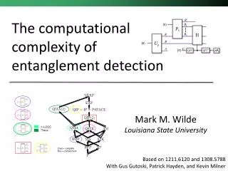
The computational complexity of entanglement detection Mark M. Wilde Louisiana State University Based on 1211.6120and 1308.5788 With Gus Gutoski, Patrick Hayden, and Kevin Milner
How hard is entanglement detection? • Given a matrix describing a bipartite state, is the state separable or entangled? • NP-hard for d x d, promise gap 1/poly(d) [Gurvits’04 + Gharibian ‘10] • Quasipolynomial time for constant gap [Brandao et al. ’10] • Probably not the right question for large systems. • Given a description of a physical process for preparing a quantum state (i.e. quantum circuit), is the state separable or entangled? • Variants: • Pure versus mixed • State versus channel • Product versus separable • Choice of distance measure (equivalently, nature of promise)
Entanglement detection: The platonic ideal NO α α YES β
Some complexity classes… P / BPP / BQP P / BPP / BQP = QIP(0) NP / MA / QMA NP / MA / QMA = QIP(1) AM / QIP(2) Cryptographic variant: Zero-knowledge Verifier, in YES instances, can “simulate” prover ZK / SZK / QSZK = QSZK(2) QMA(2) QIP = QIP(3) QIP = QIP(3) = PSPACE [Jain et al. ‘09]
Pure state circuit Product output? Trace distance BQP-complete Mixed state circuit Product output? Trace distance QSZK-complete Results: States Mixed state circuit Separable output? 1-LOCC distance (1/poly) NP-hard QSZK-hard In QIP(2)
Isometric channel Separable output? 1-LOCC distance QMA-complete Isometric channel Separable output? Trace distance QMA(2)-complete Results: Channels Noisy channel Separable output? 1-LOCC distance QIP-complete
Pure state circuit Product output? Trace distance BQP-complete Mixed state circuit Product output? Trace distance QSZK-complete Results: States Mixed state circuit Separable output? 1-LOCC distance NP-hard QSZK-hard In QIP(2)
Zero-knowledge (YES instances):Verifier can simulate prover output
Pure state circuit Product output? Trace distance BQP-complete Mixed state circuit Product output? Trace distance QSZK-complete Results: States Mixed state circuit Separable output? 1-LOCC distance NP-hard QSZK-hard In QIP(2)
Detecting mixed separable states ρAB close to separable iff it has a suitable k-extension for sufficiently large k. [BCY ‘10] Send R to the prover, who will try to produce the k-extension. Use phase estimation to verify that the resulting state is a k-extension.
Summary • Entanglement detection provides a unifying paradigm for parametrizing quantum complexity classes • Tunable knobs: • State versus channel • Pure versus mixed • Trace norm versus 1-LOCC norm • Product versus separable